Components#
Reno models are based on stocks and flows. A model is created by creating instances of these components and defining the corresponding equations that make them up.
The specifics on equations and how they’re constructed are discussed in more depth on the Math in Reno page, while this page primarily focuses on the higher level Flow/Stock/Variable components.
Flows#
Flows are equations that define rates of change, or represent how much material/information moves over time.
Flows are created with the reno.Flow class,
and the equation can either be directly provided in the constructor or by
setting the .eq attribute later on:
from reno import Flow, TimeRef
import reno

# create a flow with an equation of "5"
faucet = Flow(5)  # 5 units per timestep

# change the equation to vary sinusoidally with time
t = TimeRef()  # a TimeRef instance is a special type of variable that
               # always refers to the current timestep in the simulation
faucet.eq = reno.sin(t) * 2 + 5
(The ability to separately create the component and define the equation applies to Variables as well.)
Stocks#
A stock represents an accumulation of material or information, or some quantity thereof over time.
Stock equations are defined exclusively in terms of flows: in-flows (rates of material moving into the stock) and out-flows (rates of material moving out of the stock.)
Creating stocks in Reno are done via the Stock class:
from reno import Stock

tub_water_level = Stock()
Defining stock equations#
Stock equations are built by adding and subtracting in-flows and out-flows. The
basic syntax for doing this uses the += operator for in-flows and -=
operator for outflows:
from reno import Stock, Flow

my_inflow, my_outflow = Flow(), Flow()
my_stock = Stock()

my_stock += my_inflow
my_stock -= my_outflow
A slightly more readable syntax that allows constructing whole “chains” of
in-flows/out-flows overloads the >> and << operators, where the arrows
indicate the direction of a flow in relation to the stock on the other side:
from reno import Stock, Flow

inflow, midflow, outflow = Flow(), Flow(), Flow()
stock1, stock2 = Stock(), Stock()

inflow >> stock1 >> midflow >> stock2 >> outflow
Specifically a stock >> flow or flow << stock makes flow an
out-flow of stock, and stock << flow or flow >> stock makes
flow an in-flow to stock.
Chains of these >>/<< operations work because they are interpreted left
to right, and the “return” value of an individual operation is always the
right-most component, e.g. component2 in component1 >> component2.
As a result,
inflow >> stock1 >> midflow
is equivalent to:
inflow >> stock1
stock1 >> midflow
Implicit stock in-flows#
When an in-flow to a stock is set (either through += or >>/<<)
with an equation rather than just a flow, an implicit flow defined by that
equation is created and applied.
(e.g. if there’s some loss or dropped material between the outflow of one stock and the inflow for another. You could explicitly model this with two separate flows as well)
from reno import Stock, Flow

inflow, midflow, outflow = Flow(), Flow(), Flow()
stock1, stock2 = Stock(), Stock()

inflow >> stock1 >> midflow
(midflow - 3) >> stock2 >> outflow
by combining operations together on the same line with commas, you can still do a full chain-like definition when an inflow needs to be a slightly modified version:
from reno import Stock, Flow

inflow, midflow, outflow = Flow(), Flow(), Flow()
stock1, stock2 = Stock(), Stock()

inflow >> stock1 >> midflow, (midflow - 3) >> stock2 >> outflow
Using stocks in other equations#
Referencing a stock always refers to the stock’s value in the previous timestep. This allows a form of circular reference between stocks
from reno import Stock, Flow


my_flow = Flow()
my_stock = Stock()

my_stock += my_flow
my_flow.eq = 10 - my_stock
In this example, my_stock is incremented by the value of my_flow
in the current timestep t, while the value of my_flow for timestep t
is 10 minus the value of my_stock in timestep t - 1.
In other words, the equations for these would translate to:
my_stock(t) = my_stock(t-1) + my_flow(t)
my_flow(t) = 10 - my_stock(t-1)
Variables#
A variable is any other equation or value that can be referenced in flow (and other variable) equations and helps define the user-settable model parameters. Variables should be used to specify what can be modified about a simulation/what values you want to experiment with.
coffee_process = reno.Model(steps=10)
with coffee_process:
    drip_speed = reno.Variable(3.0)

    water = reno.Stock(init=100.0)
    coffee = reno.Stock()
    coffee_machine = reno.Flow(drip_speed, max=water)

    water >> coffee_machine >> coffee
In the above model, drip_speed is a variable that directly impacts the
coffee_machine flow/the rate at which coffee increases. Since it is a
free variable/not defined in terms of any other variables, it can be specified
during a model run to configure the simulation. We can run a couple simulations
and compare the final coffee stock values (at timestep 10):
>>> coffee_process(drip_speed=4.0).coffee.values[0, -1]
36.0

>>> coffee_process(drip_speed=1.0).coffee.values[0, -1]
9.0
Metrics#
Metrics are a special type of component whose equations run once at the end of a
simulation. These equations are normally used to retrieve a specific value or
run a basic analysis/measurement on something. Metrics are useful from a
convenience standpoint (making it semantically simpler to get e.g. the last
value of the coffee stock like in the previous example), since they are then
available to include in Reno’s Visualizations, but they can also be used
as targets for observed/measured values (“data”) for Bayesian Inference.
We can add a metric to the previous system to capture the final coffee amount with:
coffee_process.final_coffee_level = reno.Metric(coffee.timeseries[-1])
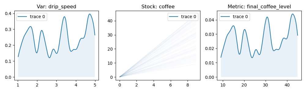
This would, for example, allow plotting the distribution of coffee produced if
an input distribution were specified for drip_speed:
>>> run = coffee_process(n=100, drip_speed=reno.Uniform(1.0, 5.0))

>>> reno.plot_trace_refs(
        coffee_process,
        [run],
        [
            coffee_process.drip_speed,
            coffee_process.coffee,
            coffee_process.final_coffee_level
        ],
        rows=1,
        cols=3,
        figsize=(10, 3)
    )
Other arguments for components#
min/max#
All stock/flow/variable components can take several optional arguments. Equation
minimum/maximum limits can be defined with values/other equations via min
and max. This can be used to constrain outflows to avoid sending a stock
into negative values (e.g. if it represents a physical quantity.) In the coffee
example above, the coffee_machine flow is initialized with a max=water,
meaning that despite the result of the equation itself, the value won’t be
greater than the available water stock in each timestep.
It is important to note that setting a min/max on a stock does not modify inflow values to that stock. To highlight this, the system below defines two stocks with a flow in between:
m = reno.Model()
with m:
    s1 = reno.Stock(init=100)
    s2 = reno.Stock(max=10)
    f1 = reno.Flow(20, max=s1)

    s1 >> f1 >> s2
s2 isn’t allowed to contain more than 10, but the inflow is pulling in 20 at
each timestep. Running this model for a few steps, we observe that s2 never goes
above 10, but s1 still decreases by 20 each time, resulting in “dropped” material.
>>> run = m(steps=3)
>>> run.s1.values[0]
array([100, 80, 60])

>>> run.f1.values[0]
array([20, 20, 20])

>>> run.s2.values[0]
array([0, 10, 10])
To appropriately bottleneck a stock like this entails also applying limits to the flow, achievable with something like the space operation discussed on the Math in Reno page.
dim/dtype#
Specifying the dtype (by passing a regular python type such as float,
int, bool, etc.) of a component ensures the type of the underlying value
and will automatically convert values as needed. This type assignment occurs on
initial value population - either automatically at the beginning of a
simulation, or by calling populate() yourself:
>>> a = r.Variable(5, dtype=float)
>>> a.eval()
5

>>> a.populate(1, 1)
>>> a.eval()
5.0
Type information is automatically determined/broadcast when not explicitly specified, and converted appropriately when it is:
>>> m = r.Model()
>>> m.a = r.Variable(5)
>>> m.b = r.Variable(m.a)
>>> m.a.dtype, m.b.dtype
(int, int)

>>> m = r.Model()
>>> m.a = r.Variable(5, dtype=float)
>>> m.b = r.Variable(m.a)
>>> m.a.dtype, m.b.dtype
(float, float)

>>> m = r.Model()
>>> m.a = r.Variable(5, dtype=float)
>>> m.b = r.Variable(m.a, dtype=int)
>>> m.a.dtype, m.b.dtype
(float, int)
dim refers to an optional “data dimension” which allows you to work with
vector data. Operations automatically broadcast according to numpy rules (TODO:
link broadcasting):
>>> a = r.Variable(5, dim=4)
>>> a.eval()
array([5, 5, 5, 5])
Note that manually specifying dim only applies if the value is not already
vectorized:
>>> a = r.Variable([5, 2], dim=4)
>>> a.eval()
array([5, 2])
cgroup/group#
cgroup and group parameters are used for controlling diagram rendering,
see Groups/Color groups.