Bayesian Inference#

Reno provides a mechanism for taking a model with multiple probability distributions and running Bayesian inference based on one or more observed values in the system in order to produce posterior probability distributions.

This is done through the PyMC library - since math equations in Reno have the ability to produce a PyTensor equivalent, Reno can recreate the entire system dynamics model as a PyMC model along with the mechanisms to compute the full timeseries outputs, and then take advantage of PyMC’s samplers to approximate posterior distributions.

The value of doing this through Reno as opposed to directly through PyMC is due to a few reasons:

Running a Reno model with PyMC is very similar to a normal run by using the model’s .pymc() call. This acts similarly to the model’s __call__(), optionally taking any free variable/initial value conditions, plus some pymc-specific sampling arguments.

A normal “forward-run” of the model using PyMC, or running the simulations just based on prior probabilities can be done by specifying the compute_prior_only=True argument.

import reno

t = reno.TimeRef()
tub = reno.Model("tub", steps=30, doc="Model the amount of water in a bathtub based on a drain and faucet rate")
with tub:
    faucet, drain = reno.Flow(), reno.Flow()
    water_level = reno.Stock()

    faucet_off_time = reno.Variable(5, doc="Timestep to turn the faucet off in the simulation.")

    faucet >> water_level >> drain

    # the faucet should be some waterflow amount until the faucet is turned
    # off, so we use a piecewise operation to make a conditional based on time
    faucet.eq = reno.Piecewise([5, 0], [t < faucet_off_time, t >= faucet_off_time])

    drain.eq = reno.sin(t) + 2
    # the drain can't move negative water, and can't drain more than exists
    # in the tub
    drain.min = 0
    drain.max = water_level

    final_water_level = reno.Metric(water_level.timeseries[-1])

trace = tub.pymc(n=1000, faucet_off_time=reno.Normal(10, 5), compute_prior_only=True)

.pymc calls return Arviz InferenceData objects, which contain a .prior XArray dataset (very similar to what the normal Reno model call returns) and when not passing compute_prior_only=True a .posterior XArray dataset as well.

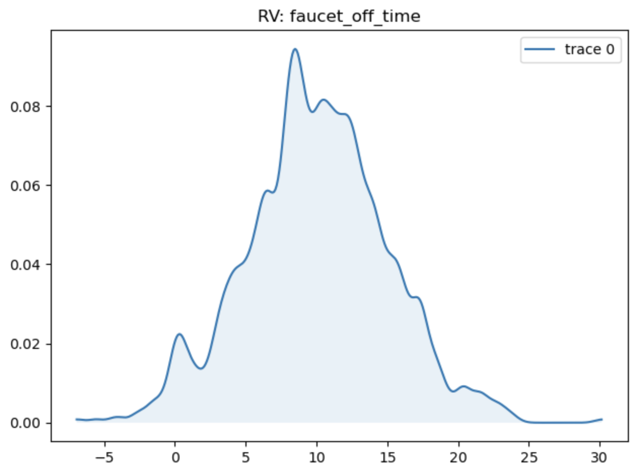
We can confirm the normal distribution on the variable by plotting it from the trace:

reno.plot_trace_refs(tub, [trace.prior], [tub.faucet_off_time])

Bayesian inference comes in when we know some additional piece of data or have an observed value for a metric somewhere, and want to determine how the probability distributions change to produce that observed value. These are provided to the .pymc call through the observations argument, which takes a list of reno.ops.Observation instances. These effectively define a normal likelihood function around a metric, with specified observed mean and standard deviation.

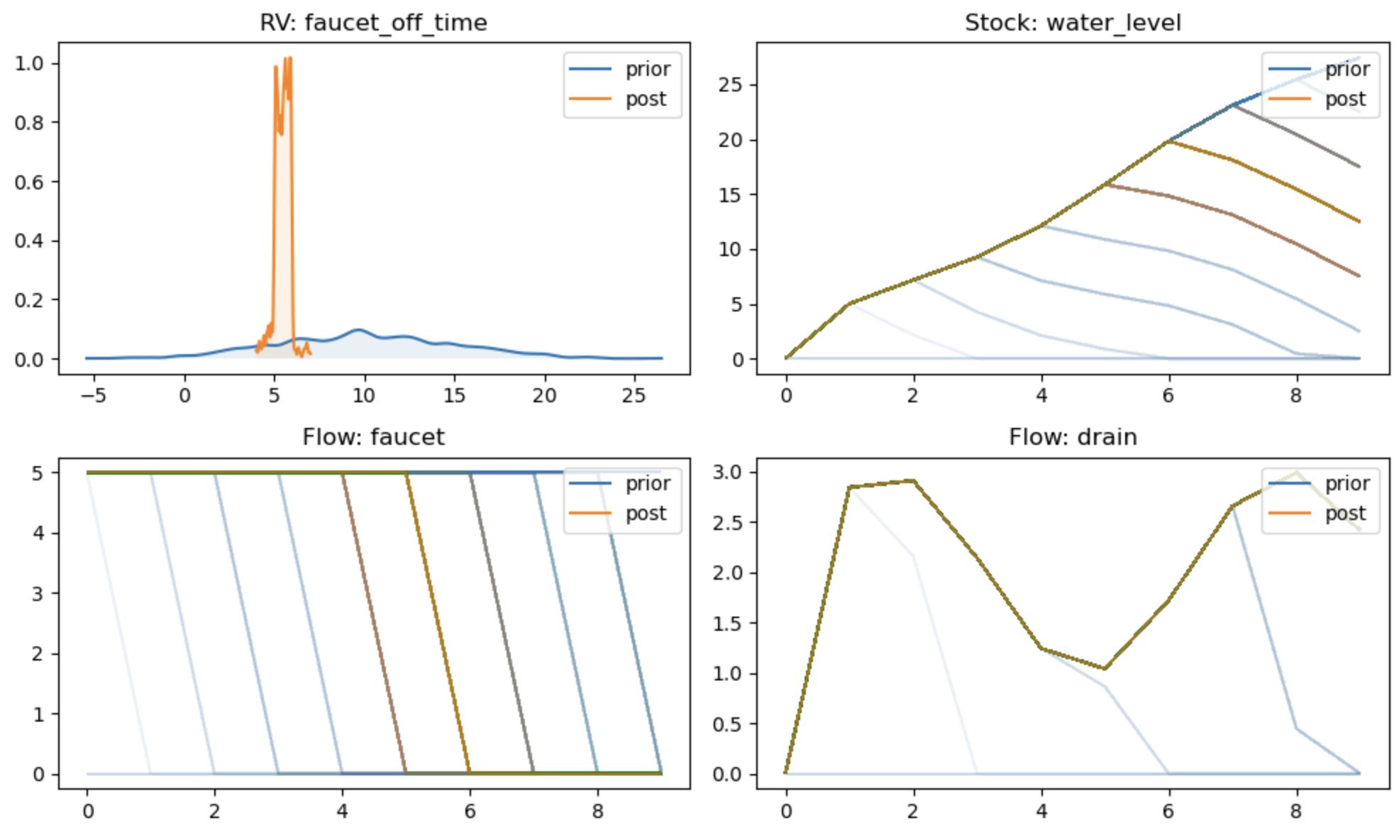
As an example, suppose we observed that the final level in the tub was 12, with some allowance for uncertainty, and we want to find out what the likely cut off time for the faucet was. We run the .pymc function with an observation on the final_water_level metric:

trace = tub.pymc(
    n=1000,
    faucet_off_time=reno.Normal(10, 5),
    observations=[reno.Observation(tub.final_water_level, 2.0, [12.0])]
)

And observe the change from prior to posterior:

reno.plot_trace_refs(
    tub,
    {"prior": trace.prior, "post": trace.posterior},
    [tub.faucet_off_time, tub.faucet, tub.drain, tub.water_level],
    figsize=(10, 6)
)

Technical process#

Under the hood, Reno produces the PyMC model made up of the following things:

A PyMC variable per component set to the initial conditions/values of that component. (When no separate init is provided for a component, this is just the equation itself run at timestep 0)
The full timeseries sequences for each component are iterated/produced using PyTensor’s scan function, inside of which runs the difference equation for every component (produced recursively through EquationPart’s .pt())
Initial conditions and timeseries sequences are combined, and any metric equations are defined as additional PyMC deterministics.
Reno adds any likelihood functions for provided observations, using normal distributions around the specified metric.

Some of the details and code samples for what this looks like can be found in the reno.pymc module.

TODO: describe the scan arguments in more depth?

Transpiling#

In addition to directly producing a PyMC model, Reno models can also transpile into a raw string of python code that creates the equivalent PyMC model. This is useful for a couple reasons - if you need to run a more complex bayesian problem than a Reno model provides (e.g. more complicated/custom likelihood functions, performance optimizations that require manual adjustment, or using the Reno model in some larger overarching model), then Reno can be used as a starting point for writing the code (and takes care of a lot of the complexity around using the scan function.) It can also be helpful for debugging issues in a PyMC model - if you’ve implemented a custom Reno operation (TODO: link to extending) and a pytensor conversion isn’t working correctly, minor changes to the PyMC code might be tested more quickly than modifying the Reno operation code first.

For example, the transpiled code from the model above produced by running print(tub.pymc_str()) (see function documentation for reno.model.Model.pymc_str()):

def tub_step(*args):
    t = args[0]
    water_level = args[1]
    faucet = args[2]
    drain = args[3]
    faucet_off_time = args[4]

    # Difference/recurrence equations
    water_level_next = (water_level + (faucet - drain))
    drain_next = pt.maximum(pt.minimum((pt.sin(t) + pt.as_tensor(2)), water_level_next), pt.as_tensor(0))
    faucet_next = pt.switch((t < faucet_off_time), pt.as_tensor(5), pt.as_tensor(0))

    # Type checks
    water_level_next = water_level_next.astype(water_level.dtype) if water_level_next.dtype != water_level.dtype else water_level_next
    drain_next = drain_next.astype(drain.dtype) if drain_next.dtype != drain.dtype else drain_next
    faucet_next = faucet_next.astype(faucet.dtype) if faucet_next.dtype != faucet.dtype else faucet_next

    return [water_level_next, faucet_next, drain_next], pm.pytensorf.collect_default_updates(inputs=args, outputs=[water_level_next, faucet_next, drain_next])

coords = {
    "t": range(10),
}
with pm.Model(coords=coords) as tub_pymc_m:
    # Initial values/timestep 0 equations
    water_level_init = pm.Deterministic("water_level_init", pt.as_tensor(np.array(0.0)))
    drain_init = pm.Deterministic("drain_init", pt.maximum(pt.minimum((pt.sin(pt.as_tensor(0)) + pt.as_tensor(2)), water_level_init), pt.as_tensor(0)))
    faucet_off_time = pm.Deterministic("faucet_off_time", pt.as_tensor(5))
    faucet_init = pm.Deterministic("faucet_init", pt.switch((pt.as_tensor(0) < faucet_off_time), pt.as_tensor(5), pt.as_tensor(0)))
    timestep_seq = pt.as_tensor(np.arange(1, 10))

    # Run autoregressive step function/timestep-wise updates to fill sequences
    [water_level_seq, faucet_seq, drain_seq], updates = pytensor.scan(
        fn=tub_step,
        sequences=[timestep_seq],
        non_sequences=[faucet_off_time],
        outputs_info=[water_level_init, faucet_init, drain_init],
        strict=True,
        n_steps=9
    )

    # Collect full sequence data for all stocks/flows/vars into pymc variables
    water_level = pm.Deterministic("water_level", pt.concatenate([pt.as_tensor([water_level_init]), water_level_seq]), dims="t")
    faucet = pm.Deterministic("faucet", pt.concatenate([pt.as_tensor([faucet_init]), faucet_seq]), dims="t")
    drain = pm.Deterministic("drain", pt.concatenate([pt.as_tensor([drain_init]), drain_seq]), dims="t")
    final_water_level = pm.Deterministic("final_water_level", water_level[pt.as_tensor(-1)])

The above output code assumes certain imports already exist (e.g. pymc and pytensor), these assumptions can also be retrieved as a string using reno.pymc.pymc_model_imports():

>>> print(reno.pymc.pymc_model_imports())
import pytensor
import pytensor.tensor as pt
import pymc as pm
import numpy as np

Bayesian Inference#

Technical process#

Transpiling#

This Page