Math in Reno#
A system dynamics model allows exploration of the behavior of a set of equations describing information or material flow over time. Reno provides a framework for creating and evaluating these equations similar to something like PyMC or PyTorch - symbolically setting up a form of compute graph that can then be populated with different values/data and evaluated over time to create simulations.
The math API itself looks similar to numpy, but a lot of the functions are being added as I go/need them, if you need a numpy function that doesn’t yet exist in Reno, please submit an issue! (Or add them yourself locally in your project, see Custom operations)
All aspects of models and their equations are made up of Reno’s
reno.components.EquationPart class, essentially a tree data
structure that can have other EquationParts as children and has an
.eval() function to
populate and execute the equation compute graph.
Execution of an equation triggers recursive .eval() calls throughout the
full tree, each component running corresponding numpy operations
on the results from its sub-equation parts.
A simple example for an equation adding two constants is shown below:
>>> eq = reno.Scalar(3.0) + reno.Scalar(2.0)
>>> eq
(+ Scalar(3.0) Scalar(2.0))

>>> type(eq)
reno.ops.add

>>> eq.sub_equation_parts
[Scalar(3.0), Scalar(2.0)]
(Note that the repr for any equation part is a lisp-like prefix-notation string, this
is used and parsed for model saving/loading.)
eq in the code above is the “root” of an equation tree, in this case an addition
operation (reno.components.Operation is a subclass of
EquationPart) which has two child nodes (“sub equation parts”), each a constant scalar value.
No math has actually occurred yet, to execute you can run eq.eval(), which
recursively evaluates through the equation tree and returns the equation value. (A
Scalar simply evaluates to its assigned
value.)
>>> eq.eval()
5.0
Reno automatically converts constants into a Scalar when it sees them, so the
following are all equivalent:
>>> reno.Scalar(3.0) + reno.Scalar(2.0)
(+ Scalar(3.0) Scalar(2.0))

>>> reno.Scalar(3.0) + 2.0
(+ Scalar(3.0) Scalar(2.0))

>>> 3.0 + reno.Scalar(2.0)
(+ Scalar(3.0) Scalar(2.0))
(at least one Reno component/operation is required for this to work, otherwise Python just evaluates the math as normal.)
Operations#
Symbolic operations, like the addition shown above, are the core of how Reno’s math
system works. A full list can be found at reno.ops. Conceptually
Reno’s math is intended to act similarly to PyTensor (what PyMC uses under the hood),
though in our implementation acting as a thunk for Numpy operations, while also providing
a way to translate directly into the PyTensor math system for Bayesian Inference reasons.
Reno’s operations are a growing list of mappings to various numpy functions, but there are some special types of operations and considerations discussed below.
As shown above, Reno operations overload many common python operators
when Reno components are involved, (e.g. +, -, *, /,
%, <, >, <=, >=, &, |), but these operations (and
the rest) are subclasses of Operation and can all be used directly by
instantiating them with the appropriate operands:
>>> reno.Scalar(3) + reno.Scalar(2) - reno.Scalar(1)
(- (+ Scalar(3) Scalar(2)) Scalar(1))

>>> reno.sub(reno.add(3, 2), 1)
(- (+ Scalar(3) Scalar(2)) Scalar(1))
Timeseries and series operations#
Reno has several operations that work across a series rather than a single
sample value. These include reno.ops.series_min/reno.ops.series_max,
reno.ops.slice, reno.ops.sum, etc. These operations can
be applied directly to values that already have an additional dimension, (TODO:
link to components multidim) for example:
>>> reno.Scalar([1, 2, 3]).sum().eval()
6

>>> reno.Variable(5, dim=3).sum().eval()
15
The normal python indexing/slicing syntax with [] can be applied
to any EquationPart and it will be turned into the appropriate Reno
operation:
>>> my_scalar = reno.Scalar([1, 2, 3])
>>> my_scalar[1]
(index Scalar([1, 2, 3]) Scalar(1))

>>> my_scalar[1].eval()
array(2)

>>> my_scalar[1:3]
(slice Scalar([1, 2, 3]) Scalar(1) Scalar(3))

>>> my_scalar[1:].eval()
array([2, 3])
Series operations can also act across a component’s values over time, done by
running the reno.ops.orient_timeseries operation on the component,
or the more semantically friendly way by calling the component’s timeseries property. This is
often useful in Metric equations, but
it can also be used in flows/variables if a flow should be based on some set of
past values. Note that during a simulation run, the timeseries is the full
length of the simulation, but all values after the current timestep are populated
with 0’s.
>>> m = reno.Model()
>>> t = reno.TimeRef()
>>> with m:
>>>     increase_over_time = reno.Variable(t + 2)
>>>     total_accumulation = reno.Variable(increase_over_time.timeseries.sum())
>>> results = m()

>>> results.increase_over_time.values
array([[ 2,  3,  4,  5,  6,  7,  8,  9, 10, 11]])

>>> results.total_accumulation.values
array([[ 2,  5,  9, 14, 20, 27, 35, 44, 54, 65]])
Historical values#
Related to the timeseries operation is the HistoricalValue component, retrieved through any component’s
history() function. This
allows specifying an index equation to retrieve a single previous value in that
component’s timeseries. For non-metric equations that don’t require slices from
the timeseries this approach should be
preferred, as any index equation that takes the form [TimeRef] - [static
value] results in a significantly simpler (and faster) PyMC output.
In general then, single previous timeseries values in stock/flow/variable equations should take the form:
t = reno.TimeRef()
my_flow.eq = my_stock.history(t - 3)
while any metric equations or stock/flow/variable equations that require more complex indexing or slicing should take the timeseries form:
t = reno.TimeRef()
some_var = reno.Variable()
my_flow.eq = my_stock.timeseries[t - some_var:t - 1].sum()
Component references#
All Components (stocks, flows, variables) inherit from EquationPart
and can be referenced/used directly inside of equations to get their current
value in a simulation:
>>> my_model = reno.Model()
>>> with my_model:
>>>     variable1 = reno.Variable(reno.Scalar(5) + 2)
>>>     variable2 = reno.Variable(variable1 + 3)

>>> # evaluating variable 2 evaluates the equation tree: ((5 + 2) + 3)
>>> my_model.variable2.eval()
10
Extended operations#
Extended or “higher order” operations are any operations that either wrap some
set of hidden sub-components or are based on other Reno operations in order to
run some more complex process. A simple example of this would be the
reno.ops.pulse operation, which returns a 1 for a specified number
of timesteps at a specified start time, and 0 at any other timestep. To achieve
this, it uses a Piecewise component rather than directly defining a
numpy/pytensor operation.
More complex examples include higher order material delays such as
reno.ops.delay1 and reno.ops.delay3, both of which
require using one or more “implicit”/inner stocks to allow accumulation of
material flowing through the op while ensuring none is lost (e.g. the total
amount of material that flows in = the total amount of material that eventully
flows out.) Components created in ExtendedOperation instances set a special implicit attribute to True, so that they
aren’t separately rendered in diagrams/latex equations etc.
Meta operations#
Meta operations are any that set up their underlying equations at runtime or instruct Reno to handle something in a specific way.
inflow#
reno.ops.inflow is a purely semantic operation that tells Reno to
treat a flow used in another flow equation as an “inflow”, as if it were a
stock. This doesn’t change the math or underlying equation, it only modifies how
the stock and flow diagram gets rendered – the thicker inflow/outflow line gets
applied to the flow to flow reference edge, which in some cases can help maintain
consistency in visualizing how material is moving in the overarching structure.
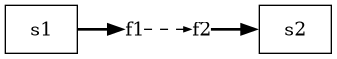
As an example, suppose we have a system with two stocks, and two flows in between them:
m = reno.Model()
with m:
    s1, s2 = reno.Stock(), reno.Stock()
    f1, f2 = reno.Flow(), reno.Flow()

    s1 >> f1
    f2.eq = f1 - 1  # some material lost between s1 and s2
    f2 >> s2
At a high level, stuff from s1 is flowing into s2 through f1 but
with some amount of loss in between, handled by f2. The thick material edges
from s1 moving to s2 is then shown indirectly, since Reno doesn’t know
if f2 is just referencing f1 in its equation, or modfiying it as an
inflow to s2. This indirectness is apparent in the diagram:
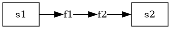
Wrapping a flow reference with inflow(), e.g. f2.eq = reno.inflow(f1)
tells Reno to render the f1 -> f2 edge as a normal flow/stock line:
m = reno.Model()
with m:
    s1, s2 = reno.Stock(), reno.Stock()
    f1, f2 = reno.Flow(), reno.Flow()

    s1 >> f1
    f2.eq = reno.inflow(f1) - 1
    f2 >> s2
Resulting in a more representative diagram:
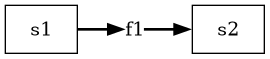
It is worth noting that for some situations this can also be achieved more
cleanly using Implicit stock in-flows, where f2 is entirely cut out
as an explicit flow, and the diagram renders more simply:
m = reno.Model()
with m:
    s1, s2 = reno.Stock(), reno.Stock()
    f1 = reno.Flow()

    s1 >> f1
    (f1 - 1) >> s2
with a more straightforward diagram:
outflows#
reno.ops.outflows is a convenience operation to provide the sum of
all outflows from a stock. This is distinct from manually constructing an
equation based on stock.out_flows because reno.ops.outflows
evaluates stock.out_flows at evaluation time rather than at the point of the
equation’s definition. The manual construction, in order to be accurate, would
have to occur after all outflows for the stock have already been defined and
attached.
More semantically, you can use this operation by referring to the property on
stocks: stock.outflows.
space#
stock.space is a property that returns
an operation (not a operation in and of itself) to help with setting up
bottlenecks on inflows. The operation returns the difference between a stock’s
value and it’s maximum allowable value, after taking the outflows for that
timestep into account. (In other words stock.max - stock + stock.outflows).
This represents the maximum value that inflows should provide to keep the stock at or below it’s maximum.
To demonstrate, the following is an updated version of the problem specified in
the min/max description regarding flow bottlenecks. We set the maximum of
the flow to take s2’s remaining space into account:
import reno as r

m = r.Model()
with m:
    s1 = r.Stock(init=100)
    s2 = r.Stock(max=10)
    f1 = r.Flow(20, max=r.minimum(s1, s2.space))

    s1 >> f1 >> s2
With the above configuration, f1 will never be greater than either s1’s
remaining value or the amount that s2 can handle in any given timestep:
>>> run = m(steps=3)
>>> run.s1.values[0]
array([100, 90, 90])

>>> run.f1.values[0]
array([10, 0, 0])

>>> run.s2.values[0]
array([0, 10, 10])
Shape and type info#
(cover multidim here)
Broadcasting#
(TODO)