Getting Started#
Installation#
Reno’s package name is reno-sd (reno was already taken) and is available
on both PyPI and conda-forge.
To install via pip:
pip install reno-sd
To install from conda-forge:
conda install conda-forge::reno-sd
The module itself is called reno and is simply imported as:
import reno
Defining a model#
Create a model by instantiating the reno.Model class,
optionally providing a name, simulation sample settings (steps - how many
timesteps to run each sample for, and n - the number of samples to run in
parallel), and an optional doc description of the model.
import reno

tub = reno.Model()

# or alternatively with more detail:
tub = reno.Model("tub", steps=30, doc="Model water flowing in/out of a bathtub")
Note that steps and n can be modified when the model is run, this simply
sets the defaults.
Adding stocks, flows, and variables to the model can be done by directly setting attributes on the model to instantiated components.
t = reno.TimeRef()  # TimeRefs are variables that always equal current timestep

# make a user-controllable variable for flow rate
tub.faucet_flow_rate = reno.Variable(6.0)

# make in and out flows
tub.faucet = reno.Flow(tub.faucet_flow_rate)
tub.drain = reno.Flow(reno.sin(t) * 2 + 4)

# make a stock to represent the accumulation of water
tub.water_level = reno.Stock()

# hook up the in and out flows to the stock
tub.water_level += tub.faucet
tub.water_level -= tub.drain
Note that since components may need to reference other components that haven’t
been created yet, the equations for flows and variables can be defined
separately from instantiation by setting the .eq attribute:
tub.faucet = reno.Flow()
tub.faucet_flow_rate = reno.Variable()

tub.faucet.eq = tub.faucet_flow_rate + 3
tub.faucet_flow_rate.eq = 5
For more info on how equations in Reno work and how to construct them, see Math in Reno.
Model with blocks#
It can be annoying to add a lot of components to a model, especially if the
model has a long variable name. Models can be used as context managers, and so
can be used in with blocks (similar to how PyMC models are conventionally
defined.) Any components defined within a model’s with block are automatically added to the
model using the components’ variable names when the context manager exits.
import reno

my_long_model_name = reno.Model()
with my_long_model_name:
    faucet_rate = reno.Variable(6.0)
    facuet = reno.Flow(faucet_rate + 3)
    drain = reno.Flow(7.0)

    water_level = reno.Stock()

    drain.max = water_level

    faucet >> water_level >> drain

# my_long_model_name now has component attributes like previous examples:
# my_long_model_name.drain
Note that the >> or << syntax as shown in the example above can be used
to simplify hooking up stock inflows and outflows, see
Defining stock equations for more details.
Inspecting a model#
The methods discussed below will be based on this example (which can also be found in the `tub notebook<https://github.com/ORNL/reno/blob/main/notebooks/tub.ipynb>`_)
import reno

t = reno.TimeRef()
tub = reno.Model("tub", doc="Model the amount of water in a bathtub based on a drain and faucet rate")
with tub:
    faucet, drain = reno.Flow(), reno.Flow()
    water_level = reno.Stock()

    faucet_off_time = reno.Variable(5, doc="Timestep to turn the faucet off in the simulation.")

    faucet >> water_level >> drain

    # the faucet should be some waterflow amount until the faucet is turned
    # off, so we use a piecewise operation to make a conditional based on time
    faucet.eq = reno.Piecewise([5, 0], [t < faucet_off_time, t >= faucet_off_time])

    drain.eq = reno.sin(t) + 2
    # the drain can't move negative water, and can't drain more than exists
    # in the tub
    drain.min = 0
    drain.max = water_level
Stock and flow diagrams#
Once a model is created, there are a few different ways to see what it looks
like. A stock and flow diagram is the easiest way to see how everything is
connected in the model, and can be generated using the model.graph()
function.
tub.graph()
The stock and flow diagram of this model looks like:
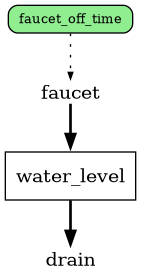
In these diagrams, the rectangular boxes represent stocks, labels between arrows represent flows, and the green rounded boxes represent variables. The heavy solid arrows represent stock in/out flows, while dashed and dotted lines indicate which references are used in which other references.
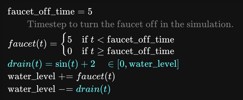
Latex equations#
A latex version of the equations for all of the stocks, flows, and variables can
be viewed with the model.latex() function.
By default this outputs (when running in Jupyter) an interactive widget with the
latex equations, and when clicking on any line, the reference name for that equation
line is highlighted everywhere else in the other equations. (This makes it
easier to track down where variables are used in very large systems.)
To get just a string version of the latex, pass raw_str=True.
Model docstring#
Models and every reference you add to models can be provided a doc
attribute, describing what the reference is/how to use it. All of this
information for a whole model can be compiled into a single Python-like
docstring using the model.get_docs()
function. This docstring shows how to configure and run the model, discussed in
the following section.
>>> print(tub.get_docs())
Model the amount of water in a bathtub based on a drain and faucet rate

Example:
    tub(faucet_off_time=5, water_level_0=None)

Args:
    faucet_off_time: Timestep to turn the faucet off in the simulation.
    water_level_0
Running a model#
Once a model is defined, it’s time to run some simulations!
A model can be called like a function, with parameters for any free variables in
the system (including any initial values for stocks) and optionally
run-specific parameters such as the number of timesteps (steps) and the
number of instances to run in parallel (n).
In the model we defined above, there’s one free variable (faucet_off_time) and
a stock initial value, water_level_0 that can be set. (These can also be
found by running tub.free_refs(), which
returns a list of string names for the free variables/initial values.
Passing values for any of these are optional, the model will rely on values provided during definition if none are provided in the call itself.
To run one instance of the tub model with all default values, use:
results = tub()
To run five instances in parallel for a longer time and different configuration:
results2 = tub(n=5, steps=100, faucet_off_time=40, water_level_0=10.0)
The return from a simulation run is an XArray dataset, containing the values of every stock/flow/variable at each timestep.
>>> print(results)
<xarray.Dataset> Size: 336B
Dimensions:          (sample: 1, step: 10)
Coordinates:
  * sample           (sample) int64 8B 0
  * step             (step) int64 80B 0 1 2 3 4 5 6 7 8 9
Data variables:
    water_level      (sample, step) float64 80B 0.0 5.0 7.159 ... 10.45 7.457
    faucet           (sample, step) int64 80B 5 5 5 5 5 0 0 0 0 0
    drain            (sample, step) float64 80B 0.0 2.841 2.909 ... 2.989 2.412
    faucet_off_time  (sample) int64 8B 5
Attributes:
    faucet_off_time:  Scalar(5)
    water_level_0:    0
As seen above, variables that are static values (e.g. faucet_off_time) don’t
include the step dimension, since they don’t change over time. A copy of the values
of each free variable in that run’s configuration are included in the
Attributes section of the output.
Running with distributions#
Running a model thus far with an n/samples more than 1 hasn’t made much sense since
these models are deterministic - each sample should run the exact same way. Samples come
into play when distributions are used in variables, which are randomly drawn from
for each sample (and optionally each timestep.) The simplest “distribution”
(which isn’t techncially a distribution) is reno.ops.List, which
simply iterates which item is selected for each sample, making it easier to
quickly test multiple variable values:
>>> tub.final_water_level = reno.Metric(tub.water_level.timeseries[-1])
>>> results = tub(n=3, faucet_off_time=reno.List([2, 4, 6]))
>>> results.final_water_level.values
array([ 0.      ,  2.456909, 12.456909])
Looking at the water level in the final timestep is now different in each sample, corresponding to the different faucet off time in each simulation.
Actually random distributions are currently available through:
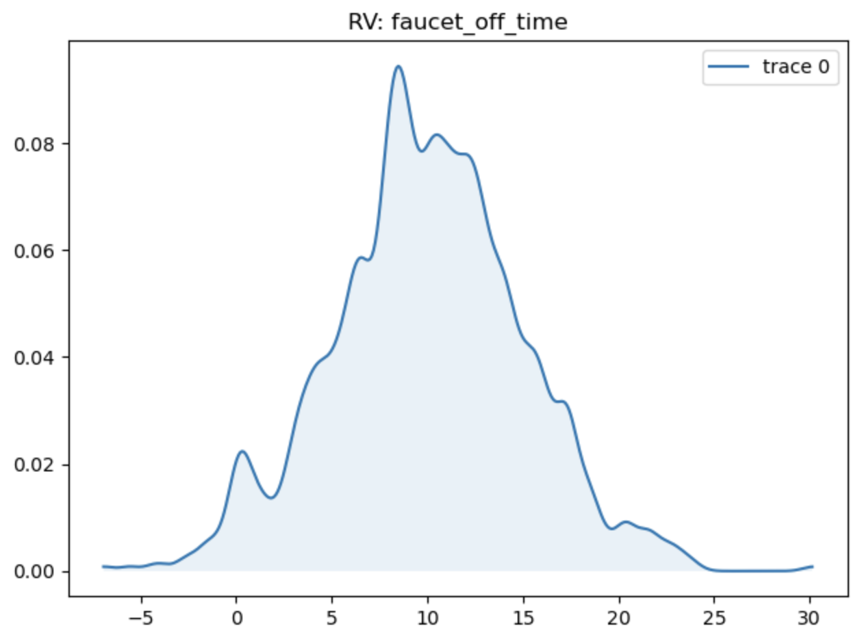
As an example, we can run the tub model with a Normal distribution with mean 10 and a standard deviation of 5 with:
>>> random_results = tub(n=1000, faucet_off_time=reno.Normal(10, 5))
>>> reno.plot_trace_refs(tub, [random_results], ["faucet_off_time"])
Systems with probability distributions can be optimized with respect to observed data, see the Bayesian Inference page for more details.
The rest of this guide#
See the other pages in the user guide for topics of interest!
Components - provides a more in depth description of stock/flow/variable components and how to define them.
Math in Reno - explains how the underlying math system works and more details on how to make equations.
Bayesian Inference - shows how the PyMC integration works and how to use it to update prior probability distributions based on observed data.
Visualizations - how to create all the nifty stock and flow diagrams and the plotting helper functions that come with Reno.
Model Explorer UI - a description of the fancy web UI for playing with models and how to run it.
Submodels - learn how to make models reusable and compositional.
Extending Reno - how to add capabilities and make Reno do more than its defaults.