Projected Heat-source Calibration

calibrateHeatSource estimates the projected model’s exponential axial-shape relation from repeated measured melt-pool depths. It runs AdditiveFOAM trials for each experimental condition, builds a response curve between the trial projection shape and simulated depth, infers a local shape value with Bayesian inference using deterministic posterior quadrature, and then fits one global nSlope–nIntercept relation.

Quantity being calibrated

For the profile diameter selected by D4Sigma—areaEquivalent, major, or minor—the calibration coordinate and runtime reference aspect ratio are

\[x=\frac{2d}{D_{4\sigma}},\] \[n=\operatorname{clip}_{[0,9]}\!\left[ \texttt{nSlope}\log_2(x)+\texttt{nIntercept}\right], \qquad k=2^n.\]

Here \(d\) is the selected reference depth. The exponential projection defines how \(k\) controls the axial distribution and how the applied source depth is selected.

The local trial cases set nSlope 0, making the rendered nIntercept equal to the trial \(n\). The global fit supplies both coefficients.

Workflow

For every parameter set, the command performs two stages:

1. Render and run trial cases at selected nIntercept values, extract the maximum requested melt-pool depth, normalize measured and simulated depths by D4Sigma/2, construct a shape-preserving PCHIP response, and infer the local posterior for \(n\).
2. Fit the local posterior modes to \(n=\texttt{nSlope}\log_2(x)+\texttt{nIntercept}\) with uncertainty weighting and a soft_l1 loss, then propagate the local posterior uncertainty through repeated global refits.

The calibration operates on melt-pool depth. Other rendered parameters—such as power, speed, end time, and write interval—define each trial but are not additional calibration responses.

Inputs

The command reads four inputs:

Input	Role
config.yml	Paths, named profiles, case execution, trial design, inference, fit, and report settings
experiments.yml	Parameter mappings and repeated measured depths
Template case	Runnable AdditiveFOAM case containing rendering placeholders
Tabulated profile files	Planar intensity distributions associated with named experimental profiles

Run it from any directory with:

calibrateHeatSource --config /path/to/config.yml

Relative paths in the configuration are resolved from the directory containing config.yml; environment variables and ~ are expanded.

Configuration

paths:
  experiments: experiments.yml
  template: template
  campaign: campaign

D4Sigma: areaEquivalent
isotherm: liquidus

profiles:
  measured_beam:
    file: template/constant/beam_profile.txt

case:
  command: ./Allrun
  keep_successful: false

calibration:
  token: nIntercept
  initial_values: [0, 1, 2, 3, 4, 5, 6, 7, 8, 9]
  bounds: [0, 9]
  max_simulations_per_experiment: 10
  depth_tolerance_microns: 1.0
  posterior_std_tolerance: 0.15
  pchip_grid_points: 1000

bayesian:
  quadrature_points: 10000
  posterior_samples: 1000

final_fit:
  bootstrap_samples: 1000
  bootstrap_random_seed: 12345

report:
  enabled: true

Entry	Meaning
paths.experiments	Experimental YAML file
paths.template	Template case copied for each trial
paths.campaign	Writable trial-case and output directory
D4Sigma	Select areaEquivalent, major, or minor for the source reference width and depth normalization
isotherm	Numeric temperature or liquidus; defaults to liquidus
profiles.<name>.file	Tabulated profile associated with the name used by experiments
case.command	Command executed inside every rendered trial case
case.keep_successful	Retain or remove processor and numeric time directories after metrics are saved
calibration.token	Placeholder name rendered in the template; normally nIntercept
calibration.initial_values	Initial local trial values
calibration.bounds	Allowed bounds for initial and adaptively proposed trial values
calibration.max_simulations_per_experiment	Maximum AdditiveFOAM trials for one condition
calibration.depth_tolerance_microns	Stops adaptive refinement when a trial depth is sufficiently close to the measured mean
calibration.posterior_std_tolerance	Stops adaptive refinement when local posterior uncertainty is sufficiently small
calibration.pchip_grid_points	Grid used when proposing an additional trial from the response curve
bayesian.quadrature_points	Dense PCHIP/posterior evaluation grid
bayesian.posterior_samples	Stratified inverse-CDF samples retained for global propagation
final_fit.bootstrap_samples	Number of posterior-resampling global refits
final_fit.bootstrap_random_seed	Reproducible random seed for those refits

calibration.pchip_grid_points controls adaptive trial placement and is distinct from bayesian.quadrature_points, which controls posterior integration.

Experiments

Each entry supplies a general parameter mapping and repeated depth observations:

- parameters:
    Power_W: 187.5
    Speed_mm_s: 500
    Profile: measured_beam
  Measured_Depth_microns: [87.05, 98.10]

Profile must match a name in config.yml. The tutorial template renders Power_W, Speed_mm_s, and the calibration token, but additional parameter keys may be used when matching placeholders are added to a custom template.

Beam metrics and normalization

Before running cases, calibrateHeatSource calls tabulatedProfileInfo for every named profile. That utility reports the exact bilinear planar integral, centroid, principal second-moment diameters, and azimuth. The driver then selects major, minor, or the area-equivalent diameter

\[D_{4\sigma}=\sqrt{ D_{4\sigma,\mathrm{major}}D_{4\sigma,\mathrm{minor}}}.\]

Measured and simulated depths are both normalized as

\[y=\frac{\mathrm{Depth}}{D_{4\sigma}/2} =\frac{2\,\mathrm{Depth}}{D_{4\sigma}}.\]

The profile table supplies the reference width. The source obtains its lateral support from the tabulated profile, so the template has no rendered radius. These quantities use the profileMetrics definition.

Template requirements

The template must run independently after its placeholders are rendered. The calibration placeholder must appear once and use <<name>> syntax:

sources
{
    beam
    {
        path            scanPath;
        widthReference  D4Sigma;
        D4Sigma         <<D4Sigma>>;
        depthReference  isotherm;
        isotherm        <<isotherm>>;

        absorption
        {
            model               Kelly;
            eta0                0.27;
            etaMin              0.27;
            aspectRatioSwitch   0.0;
            geometry            cylinder;
        }

        heatSource
        {
            model       projected;
            depth       20e-6;
            nPoints     (10 10 10);

            profile
            {
                model   tabulated;
                file    "beam_profile.txt";
            }

            projection
            {
                model       exponential;
                nSlope      0;
                nIntercept  <<nIntercept>>;
            }
        }
    }
}

The named beam table is copied into each rendered case. The template also renders the selected D4Sigma component and isotherm, scan-path power and speed, end time, and write interval for the selected experiment.

When top-level isotherm is liquidus, the command expands constant/transportProperties with foamDictionary, finds the temperature paired with alpha.solid = 0 in thermoPath, renders that value into both heatSourceDict and the meltPoolDimensions function object, and reads the matching CSV.

AdditiveFOAM response curves

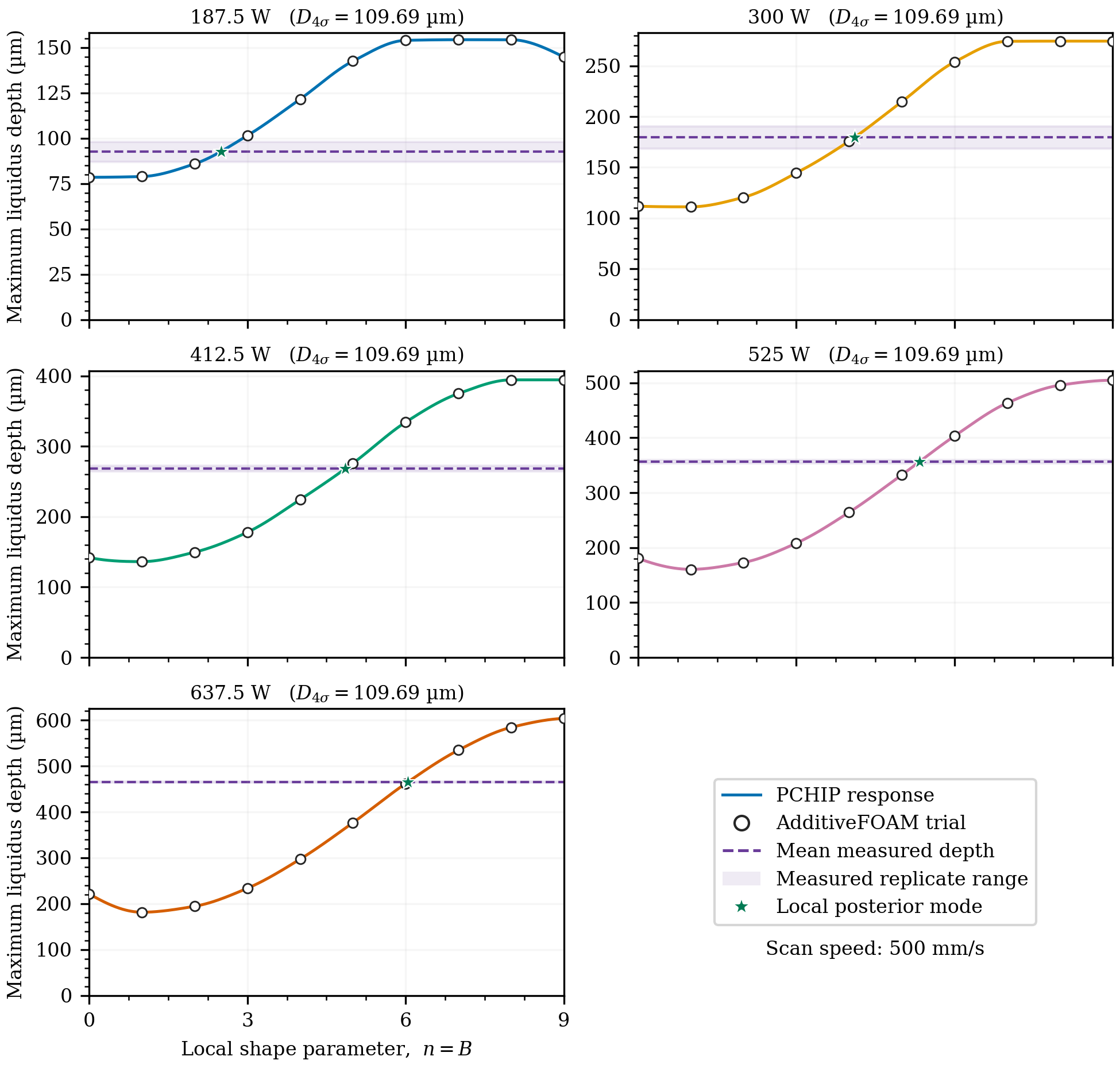
For a condition \(c\), trial runs provide pairs \((n_j,y_j^{\mathrm{AF}})\), where \(y_j^{\mathrm{AF}}\) is the normalized simulated depth. A piecewise cubic Hermite interpolating polynomial, PCHIP, constructs \(\widehat y_c(n)\) without extrapolating beyond the available trial range. PCHIP preserves the sampled curve shape and avoids the overshoot that an unconstrained cubic spline can introduce.

The configured initial values are run for a new condition. If fewer than two valid trial results exist, missing initial values are added. When the initial design leaves room below max_simulations_per_experiment, the algorithm can add a response-curve crossing near the measured mean until either the closest simulated depth is within depth_tolerance_microns, the posterior standard deviation is below posterior_std_tolerance, no crossing can be proposed, or the trial limit is reached.

Local response construction for the five tutorial conditions. Circles are the ten AdditiveFOAM trials, solid lines are the PCHIP responses, purple lines and bands show the measured mean and replicate range, and stars mark the local posterior modes.

Local Bayesian inference using deterministic posterior quadrature

For repeated normalized measurements \(\mathbf y=(y_1,\ldots,y_R)\), the local posterior is

\[p(n\mid\mathbf y)\propto p(\mathbf y\mid n)p(n).\]

The response surrogate is defined only over the available trial support

\[\mathcal S_n=[\min_j n_j,\max_j n_j].\]

The local prior is uniform on \(\mathcal S_n\) and zero outside it. All trial values must lie within calibration.bounds, and the posterior support is the span of the completed trials. Conditional on \(n\), repeated measurements are independent normal observations of the interpolated AdditiveFOAM response:

\[y_r\mid n\sim\mathcal N\!\left(\widehat y(n),\sigma^2\right),\] \[s_0(\mathbf y)= \sqrt{\frac{1}{R}\sum_{r=1}^{R}(y_r-\overline y)^2},\] \[\sigma=\max\!\left(0.05\,\overline y,s_0(\mathbf y)\right).\]

Here \(s_0\) is the population standard deviation used by NumPy’s default std calculation, with divisor \(R\).

For \(n\in\mathcal S_n\),

\[\log p(n\mid\mathbf y)=C- \frac{1}{2\sigma^2}\sum_{r=1}^{R} \left[y_r-\widehat y(n)\right]^2.\]

The implementation evaluates this density on bayesian.quadrature_points, subtracts its maximum log density for numerical stability, and normalizes it with trapezoidal integration. It then calculates:

• the mode at the maximum evaluated density;
• mean and variance by trapezoidal quadrature;
• median and equal-tail 95% credible interval from the numerical CDF;
• bayesian.posterior_samples stratified inverse-CDF samples for the global fit.

Global calibration fit

Each condition contributes the local posterior mode \(n_c\), its posterior standard deviation \(s_c\), and its measured

\[x_c=\frac{2\,\overline{\mathrm{Depth}}_c}{D_{4\sigma,c}}.\]

The global model is

\[n_c\approx\texttt{nSlope}\log_2(x_c)+\texttt{nIntercept}.\]

The fit minimizes standardized residuals

\[r_c=\frac{n_c- \texttt{nSlope}\log_2(x_c)-\texttt{nIntercept}}{ \max(s_c,s_{\min})}\]

with SciPy least_squares and a soft_l1 loss when at least three conditions are available. The uncertainty weighting gives sharper local posteriors more influence, while the loss limits the leverage of an isolated inconsistent condition. AdditiveFOAM clips the fitted prediction to \(0\leq n\leq9\).

For each bootstrap realization, the command draws one value from every stored local posterior, refits nSlope and nIntercept, and evaluates the clipped response. Pointwise 2.5% and 97.5% quantiles form the empirical 95% fit interval. If stored posterior samples are unavailable for a condition, a normal approximation based on its local mode and standard deviation is used.

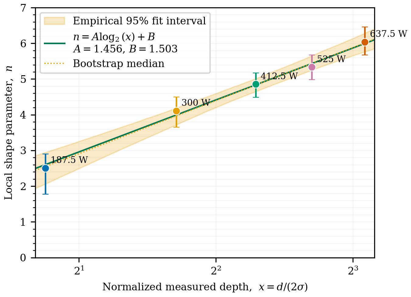
The uncertainty-weighted global calibration. Points and asymmetric error bars summarize the local posteriors, the green curve is the fitted nSlope–nIntercept relation, and the orange band propagates local uncertainty through the bootstrap refits.

Outputs

campaign/
├── cases/
├── simulations.yml
├── calibration_state.yml
├── calibration_fit.yml
└── reports/
    ├── calibration_report.pdf
    └── calibration_summary.csv

simulations.yml stores completed response trials, and calibration_state.yml stores local posterior summaries and retained samples. The command resumes from these files and recalculates results when their inputs change. calibration_fit.yml records nSlope, nIntercept, covariance diagnostics, bootstrap intervals, weighted residuals, the observed x range, and x_definition: 2*Depth / selected diameter. The summary CSV contains one row per experiment. The PDF contains profile metrics, response curves, local posterior densities, the global fit, and its uncertainty interval.

Apply the fitted values in the source dictionary:

projection
{
    model       exponential;
    nSlope     <fitted-nSlope>;
    nIntercept <fitted-nIntercept>;
}