Heat Source Models
AdditiveFOAM represents deposited energy with one or more moving volumetric sources. Each named source defines its scan path, reference dimensions, absorption model, and heat-source model. Nested dictionaries select each model with a model entry.
Source dictionary
The dictionary below configures a tabulated planar profile with an exponential axial projection:
sources
{
    beam
    {
        path            scanPath;

        widthReference  D4Sigma;
        D4Sigma         areaEquivalent; // areaEquivalent, major, or minor
        depthReference  isotherm;        // constant or isotherm
        isotherm        1620;            // optional; liquidus by default

        absorption
        {
            model       constant;        // or Kelly
            eta         0.35;
        }

        heatSource
        {
            model       projected;
            depth       20e-6;
            tolerance   1e-3;
            nPoints     (10 10 10);

            profile
            {
                model   tabulated;       // superGaussian, nLightAFX, tabulated
                file    "beamProfile.txt";
            }

            projection
            {
                model       exponential;
                nSlope      0;
                nIntercept  1;
            }
        }
    }
}

refinement
{
    model none;
}
widthReference, D4Sigma, depthReference, and isotherm are source-level entries. The heat-source and absorption models use the same reference aspect ratio.
Model hierarchy
| Level | Selections | Role |
|---|---|---|
| Source | Any user-defined dictionary name under sources |
Combines motion, reference dimensions, absorption, and volumetric deposition |
absorption |
constant, Kelly |
Converts incident scan-path power to absorbed power |
heatSource |
superGaussian, modifiedSuperGaussian, projected |
Defines the normalized three-dimensional source distribution |
projected/profile |
superGaussian, nLightAFX, tabulated |
Defines the two-dimensional beam-plane distribution |
projected/projection |
exponential |
Defines the one-sided axial distribution |
refinement |
none, targetCellLoad, timeStep, uniformTimeIntervals |
Controls scan-path-aware mesh marking |
superGaussian is both a volumetric model and a planar profile available inside projected. modifiedSuperGaussian is a volumetric model. projected combines a planar profile with an axial projection.
Source-level entries
| Entry | Required | Default | Meaning |
|---|---|---|---|
path |
Yes | — | Scan-path file under constant/ |
deltaT |
No | Unlimited | Maximum temporal source-integration interval; when configured, it is expected to be positive |
hitPathIntervals |
No | true |
Reduce solver steps as needed to land on scan-path interval ends |
widthReference |
No | D4Sigma |
Reference-width definition; only D4Sigma is supported |
D4Sigma |
No | areaEquivalent |
Select areaEquivalent, major, or minor from profileMetrics |
depthReference |
No | constant |
Select constant or isotherm reference depth |
isotherm |
No | Material liquidus | Temperature used by depthReference isotherm |
absorption |
Yes | — | Nested absorption model dictionary |
heatSource |
Yes | — | Nested volumetric heat-source dictionary |
The top-level refinement dictionary is optional and defaults to model none. See Adaptive Mesh Refinement for the other models.
Scan paths
The first line of the file selected by path is a header and is ignored. Each following non-empty row contains:
mode x y z power parameter
| Mode | Position columns | Power column | Parameter column |
|---|---|---|---|
0 |
Endpoint of a linear segment, in metres | Incident power during the segment, in watts | Translation speed, in m/s |
1 |
Fixed source position, in metres | Incident power during the dwell, in watts | Dwell duration, in seconds |
A zero-power row represents motion or dwell without deposition. The case-file reference gives the path interpolation equations.
Beam-plane profile metrics
profileMetrics characterizes the beam-plane intensity footprint of every heat-source profile. Analytic volumetric models and projected analytic profiles calculate the metrics from their distributions. A tabulated profile calculates them from its bilinear interpolant.
For a nonnegative intensity distribution \(I(x,y)\) in the source-relative beam plane, define the raw moments
\[M_{mn}=\iint x^m y^n I(x,y)\,\mathrm dx\,\mathrm dy, \qquad m+n\leq2,\]with positive integral \(M_{00}\). The centroid is
\[\bar x=\frac{M_{10}}{M_{00}},\qquad \bar y=\frac{M_{01}}{M_{00}},\]and the covariance matrix is
\[\boldsymbol\Sigma= \begin{bmatrix} M_{20}/M_{00}-\bar x^2 & M_{11}/M_{00}-\bar x\bar y\\ M_{11}/M_{00}-\bar x\bar y & M_{02}/M_{00}-\bar y^2 \end{bmatrix}.\]If \(\lambda_{\mathrm{major}}\geq\lambda_{\mathrm{minor}}\) are the eigenvalues of \(\boldsymbol\Sigma\), the stored beam diameters are
\[D_{4\sigma,\mathrm{major}}=4\sqrt{\lambda_{\mathrm{major}}}, \qquad D_{4\sigma,\mathrm{minor}}=4\sqrt{\lambda_{\mathrm{minor}}},\]ordered (major minor). The major-axis azimuth is
AdditiveFOAM reports zero azimuth for a circular profile, where orientation is undefined; numerically, it treats the eigenvalue split as circular when it is no larger than rootSmall times the mean variance, with a VSMALL floor. Each D4Sigma value is a diameter; the corresponding second-moment radius is \(D_{4\sigma}/2\).
For tabulated, AdditiveFOAM integrates all six raw moments over each table cell’s bilinear interpolant. The resulting planar integral must be positive. tabulatedProfileInfo and primesToAdditiveFoam report the same metrics.
Reference dimensions
The source-level reference-dimension settings reduce the two principal profile diameters and a selected depth to the scalar aspect ratio used by the heat-source and absorption models.
For profile principal diameters \(D_{\mathrm{major}}\) and \(D_{\mathrm{minor}}\), the selected reference width is
\[D_{\mathrm{ref}}= \begin{cases} D_{\mathrm{major}}, & \texttt{D4Sigma major},\\ D_{\mathrm{minor}}, & \texttt{D4Sigma minor},\\ \sqrt{D_{\mathrm{major}}D_{\mathrm{minor}}}, & \texttt{D4Sigma areaEquivalent}. \end{cases}\]With depthReference constant, the reference depth is the configured heat-source depth. With depthReference isotherm, AdditiveFOAM measures the maximum selected-isotherm depth below the source-relative beam plane and within the planar profile bounds. The optional isotherm value defaults to the material liquidus.
The reference aspect ratio is
\[a=\frac{2d_{\mathrm{ref}}}{D_{\mathrm{ref}}}.\]The depth actually applied to the spatial heat source is a separate quantity:
\[d_{\mathrm{source}}= \max(d_{\mathrm{configured}},d_{\mathrm{ref}}).\]The configured depth is the minimum applied depth when depthReference isotherm is selected. The heat-source distribution uses \(d_{\mathrm{source}}\). The axial projection and Kelly absorption use \(a\).

profileMetrics characterizes every planar footprint. The selected reference width and reference depth form one shared aspect ratio; the applied source depth is calculated separately.Volumetric power density
Let \(\mathbf{X}\) be a point in the global coordinate system. For source \(b\), the beam position is \(\mathbf{X}_b(t)\), and the source-relative position is
\[\mathbf{x}=\mathbf{X}-\mathbf{X}_b(t)=(x,y,z).\]The beam plane is \(z=0\), and material below it has \(z\leq0\). Each heat-source model defines a nonnegative dimensionless weight \(w_b(\mathbf{x},t)\) and its volume integral
\[\mathcal V_b(t)=\iiint_{\mathbb R^3} w_b(\mathbf{x},t)\,\mathrm dV.\]The absorbed volumetric power density is
\[\dot q_b(\mathbf{X},t)= \eta_b(a_b(t))P_b(t) \frac{w_b(\mathbf{x},t)}{\mathcal V_b(t)},\]where \(P_b\) is incident power and \(\eta_b\) is absorptivity. The normalized kernel \(w_b/\mathcal V_b\) has units of m\(^{-3}\), so \(\dot q_b\) has units of W m\(^{-3}\) and satisfies
\[\iiint_{\mathbb R^3}\dot q_b(\mathbf{X},t)\,\mathrm dV =\eta_b(a_b(t))P_b(t).\]For \(B\) sources, the field in the energy equation is
\[\dot q(\mathbf{X},t)=\sum_{b=1}^{B}\dot q_b(\mathbf{X},t).\]The analytic normalization stored by the model is V0. The spatial quadrature evaluates the cell-average weight. If its domain integral is within five percent of V0, AdditiveFOAM uses that discrete integral to remove the remaining quadrature error.
For analytic profiles with azimuth \(\theta\), define the coordinates aligned with the profile’s principal axes by
\[u=x\cos\theta+y\sin\theta,\qquad v=-x\sin\theta+y\cos\theta.\]The equations below use \(\mathbf{X}\) only for the global evaluation point, \(\mathbf{x}\) only for the source-relative position, and \((u,v)\) only for this planar rotation. The source index is omitted within each individual model equation.
Source update and temporal integration
Source state is synchronized once before temporal beam subcycling:
- Select the profile-metric reference width.
- Use the configured depth or measure the selected isotherm depth.
- Form \(a=2d_{\mathrm{ref}}/D_{\mathrm{ref}}\) and \(d_{\mathrm{source}}=\max(d_{\mathrm{configured}},d_{\mathrm{ref}})\).
- Update the heat-source shape, normalization, and retained bounds with those two quantities.
- Evaluate Kelly, when selected, with the same reference aspect ratio.
- Temporally integrate the moving source through the solver step.
For a CFD step \([t^n,t^{n+1}]\) of duration \(\Delta t^n\), the field supplied to the energy equation is the temporal average
\[\overline{\dot q}^{n}(\mathbf{X})= \frac{1}{\Delta t^n} \sum_{b=1}^{B} \int_{t^n}^{\min(t^{n+1},t_{\mathrm{end},b})} \dot q_b(\mathbf{X},t)\,\mathrm dt.\]AdditiveFOAM evaluates this integral by beam subcycling with the source-level deltaT. Division by the full CFD-step duration preserves the active-power fraction when the step extends past the end of a scan path.
All heat-source kernels are one-sided below the source-relative beam plane: they are zero for \(z>0\) and normalized over their support at \(z\leq0\).
Absorption models
constant
absorption
{
    model constant;
    eta   0.33;
}
eta is the fixed absorbed fraction of incident scan-path power.
Kelly
absorption
{
    model             Kelly;
    geometry          cone;
    eta0              0.28;
    etaMin            0.35;
    aspectRatioSwitch 1.0;
}
geometry is required and must be cone or cylinder; eta0 and etaMin are required. aspectRatioSwitch defaults to one. With source-level reference aspect ratio \(a\) and switch \(a_s\),
Above the switch, \(\beta=\tan^{-1}(1/a)\) and
\[[F,G]= \begin{cases} \left[(3\sin\beta-\sin3\beta)/4, 1/(1+\sqrt{1+a^2})\right], & \texttt{cone},\\[4pt] \left[(1-\cos2\beta)/2,1/(2(1+a))\right], & \texttt{cylinder}. \end{cases}\]At or below aspectRatioSwitch, Kelly returns etaMin before evaluating \(1/a\). Above the switch, etaMin lower-bounds the analytic curve.
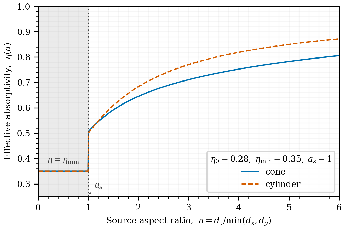
etaMin applies below the switch and lower-bounds the analytic curve above it.Heat-source entries
Every heatSource model requires scalar depth. The optional entries are:
| Entry | Default | Meaning |
|---|---|---|
tolerance |
1e-3 |
Maximum analytic source-power fraction omitted outside retained bounds |
nPoints |
(1 1 1) |
Nominal source-bound resolution used to derive per-cell midpoint sample counts |
Analytic models derive bounds from their cumulative integrals. Tabulated profiles use their exact finite nodal support. A projected source divides the total tolerance between planar and axial factors using
so \((1-\epsilon)^2=1-\texttt{tolerance}\).
For retained-bound span \(L_j\), nPoints defines a nominal spacing \(h_j=L_j/n_j\). In an overlapping hexahedral cell with bounding-box span \(\ell_{c,j}\), the implementation converts the positive ratio to an integer and enforces at least one sample:
The cell is sampled at the midpoints of the resulting uniform subdivisions. Because the ratio is integerized, nPoints establishes a nominal resolution; it does not guarantee that every actual subcell spacing is no larger than \(h_j\). Non-hexahedral cells are evaluated at the cell centre.
Volumetric models
superGaussian
heatSource
{
    model       superGaussian;
    radius      (85e-6 60e-6);
    depth       30e-6;
    definition  secondMoment;
    azimuth     25;
    k           2;
    nPoints     (10 10 10);
}
radius is a required vector2D, depth and k are required scalars, and azimuth defaults to zero degrees. definition defaults to e2 and may be e2 or secondMoment. For lateral coefficient
and the principal-axis coordinates \((u,v)\) defined above, the volumetric weight is
\[w_{\mathrm{SG}}(u,v,z)= \begin{cases} \displaystyle \exp\!\left\{-\left[ C\left(\frac{u^2}{r_x^2}+\frac{v^2}{r_y^2}\right) +2^{2/k}\frac{z^2}{d_{\mathrm{source}}^2} \right]^{k/2}\right\}, & z\leq0,\\[8pt] 0, & z>0. \end{cases}\]Its analytic volume integral is
\[\mathcal V_{\mathrm{SG}}= \frac{2\pi r_xr_y d_{\mathrm{source}}} {3C\,2^{1/k}} \Gamma\!\left(1+\frac{3}{k}\right),\]and the model supplies
\[\dot q(\mathbf{X},t)= \eta(a)P(t) \frac{w_{\mathrm{SG}}(u,v,z)} {\mathcal V_{\mathrm{SG}}}.\]Before rotation by azimuth, the principal beam-plane diameters are
The secondMoment definition makes each configured local radius one half of its corresponding D4Sigma diameter. The e2 definition makes each radius the planar distance at which the axis-aligned profile falls to \(e^{-2}\).
modifiedSuperGaussian
heatSource
{
    model       modifiedSuperGaussian;
    radius      (40e-6 40e-6);
    depth       20e-6;
    definition  e2;
    azimuth     0;
    k           7.95;
    m           2.72;
    nPoints     (10 10 10);
}
modifiedSuperGaussian uses the same radius, depth, definition, azimuth, and k entries as superGaussian and also requires m. With positive depth \(\zeta=-z\),
The beam-plane integral at \(\zeta=0\) and the three-dimensional normalization are
\[\mathcal A_{\mathrm{SG}}= \frac{\pi r_xr_y}{C} \Gamma\!\left(1+\frac{2}{k}\right),\] \[\mathcal V_{\mathrm{MSG}}= \mathcal A_{\mathrm{SG}}d_{\mathrm{source}} \frac{\Gamma(1+1/m)\Gamma(1+2/m)} {\Gamma(1+3/m)}.\]The corresponding power density is
\[\dot q(\mathbf{X},t)= \eta(a)P(t) \frac{w_{\mathrm{MSG}}(u,v,\zeta)} {\mathcal V_{\mathrm{MSG}}}.\]At \(\zeta=0\), the planar weight is \(I_{\mathrm{SG}}\). The principal D4Sigma diameters therefore follow the superGaussian expression above.
projected model
projected constructs a separable volumetric source from one planar profile \(I(x,y)\) and one axial projection \(p(z)\). Define
The normalized planar and axial kernels are
\[\phi(x,y)=\frac{I(x,y)}{\mathcal A_I}, \qquad \psi(z)=\frac{p(z)}{\mathcal A_p},\]with units m\(^{-2}\) and m\(^{-1}\), respectively. Therefore
\[w_{\mathrm{projected}}(x,y,z)=I(x,y)p(z), \qquad \mathcal V_{\mathrm{projected}}=\mathcal A_I\mathcal A_p,\]and the deposited power density is
\[\dot q(\mathbf{X},t)= \eta(a)P(t)\phi(x,y)\psi(z) =\eta(a)P(t) \frac{I(x,y)p(z)}{\mathcal A_I\mathcal A_p}.\]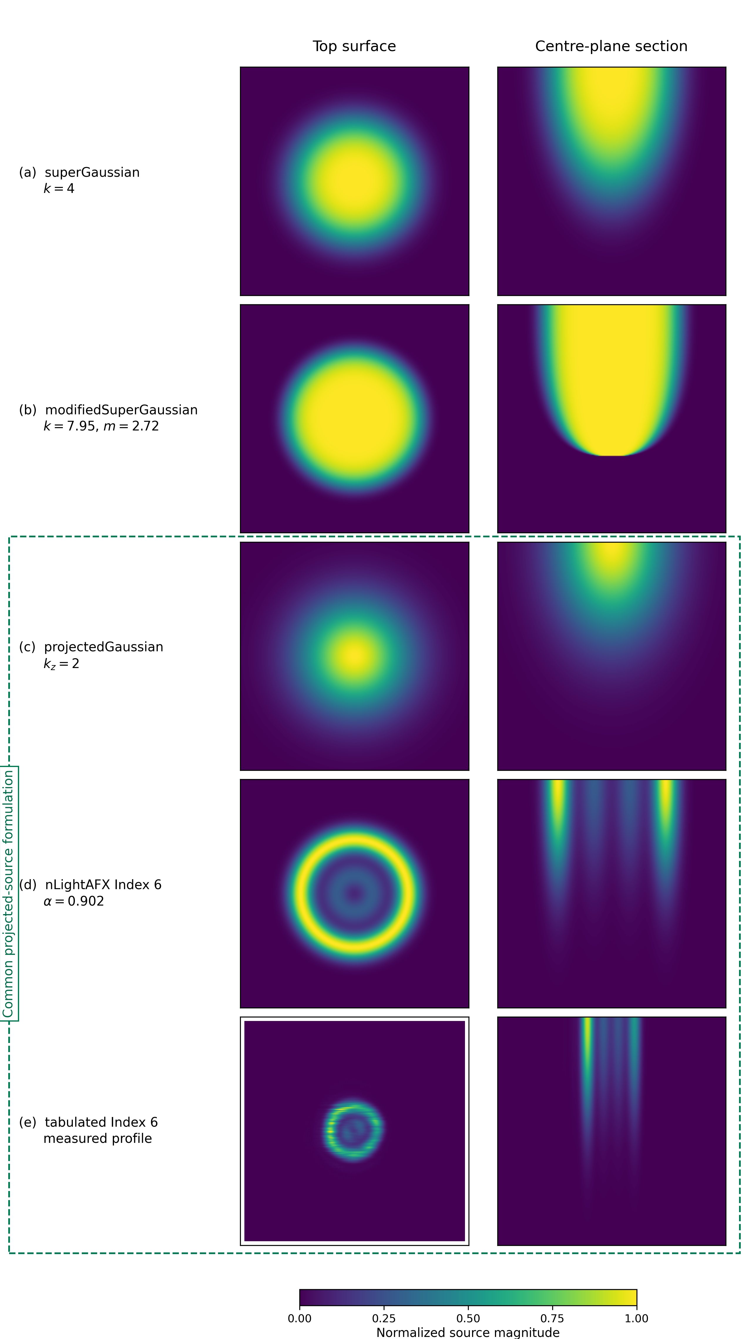
projected source combines one planar profile with the shared exponential projection.
exponential projection
The supported axial projection is:
projection
{
    model       exponential;
    nSlope      0;
    nIntercept  1;
}
For positive depth \(\zeta=-z\) and the separately calculated source depth \(d_{\mathrm{source}}\),
\[p(z)= \begin{cases} \displaystyle \exp\!\left[-3 \left(\frac{\zeta}{d_{\mathrm{source}}}\right)^k\right], & z\leq0,\\[6pt] 0, & z>0, \end{cases}\] \[n=\operatorname{clip}\!\left[ \texttt{nSlope}\log_2\!\left(\max(a,\texttt{VSMALL})\right) +\texttt{nIntercept},0,9\right], \qquad k=2^n,\] \[\mathcal A_p=\frac{d_{\mathrm{source}}\Gamma(1/k)} {k\,3^{1/k}}.\]Here \(a=2d_{\mathrm{ref}}/D_{\mathrm{ref}}\) sets the exponent, while \(d_{\mathrm{source}}\) sets the axial length scale in \(p\) and \(\mathcal A_p\).
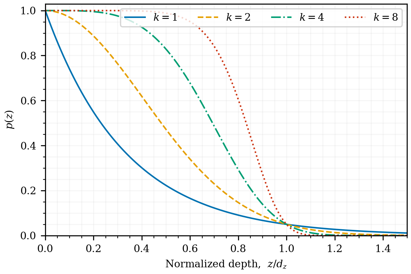
exponential projection. Increasing n, and therefore k, flattens the distribution through most of the applied depth and sharpens its edge.Use calibrateHeatSource to infer nSlope and nIntercept from measured melt-pool depths and AdditiveFOAM response curves.
superGaussian profile
profile
{
    model       superGaussian;
    radius      (55e-6 40e-6);
    definition  secondMoment;
    azimuth     25;
    k           2;
}
The planar profile uses the same required radius and k, optional definition e2|secondMoment, and optional azimuth in degrees as the volumetric model. Its weight and planar integral are
Thus \(\phi_{\mathrm{SG}}=I_{\mathrm{SG}}/\mathcal A_{\mathrm{SG}}\), and a projected source using this profile has
\[\dot q(\mathbf{X},t)= \eta(a)P(t)\phi_{\mathrm{SG}}(u,v)\psi(z).\]The principal D4Sigma diameters are given by the superGaussian expression above. The profile calculates profileMetrics analytically.
nLightAFX profile
#include "$ADDITIVEFOAM_ETC/heatSources/nLightAFX-1000.cfg"

profile
{
    model nLightAFX;
    $Index6;
}
Each shared mode supplies alpha, r0, sigma0, r1, and sigma1. For component \(i\in\{0,1\}\), \(r_i\) is the ring radius and \(\sigma_i\) is its radial standard deviation. With \(\rho=\sqrt{x^2+y^2}\), the two unnormalized ring weights are
Their radial integrals are
\[J_i=\int_0^\infty I_i(\rho)\rho\,\mathrm d\rho =2\sigma_i^2\exp\!\left(-\frac{r_i^2}{2\sigma_i^2}\right) +r_i\sigma_i\sqrt{2\pi}\, \operatorname{erf}\!\left(\frac{r_i}{\sqrt{2}\sigma_i}\right).\]Because the planar integral of component \(i\) is \(2\pi J_i\), the combined planar weight is
\[I_{\mathrm{AFX}}(\rho)= (1-\alpha)I_0(\rho) +\alpha\frac{J_0}{J_1}I_1(\rho),\]with
\[\mathcal A_{\mathrm{AFX}}=2\pi J_0.\]The normalized planar kernel is
\[\phi_{\mathrm{AFX}}(\rho)= (1-\alpha)\frac{I_0(\rho)}{2\pi J_0} +\alpha\frac{I_1(\rho)}{2\pi J_1}.\]The factor \(J_0/J_1\) gives both unweighted ring profiles the same planar integral before \(\alpha\) is applied. Equivalently,
\[\iint (1-\alpha)\frac{I_0}{2\pi J_0}\,\mathrm dA=1-\alpha, \qquad \iint \alpha\frac{I_1}{2\pi J_1}\,\mathrm dA=\alpha.\]A projected nLight AFX source is
\[\dot q(\mathbf{X},t)= \eta(a)P(t)\phi_{\mathrm{AFX}}(\rho)\psi(z).\]For the circular profile, define
\[\begin{aligned} K_i&=\int_0^\infty I_i(\rho)\rho^3\,\mathrm d\rho\\ &= 2\sigma_i^2(r_i^2+2\sigma_i^2) \exp\!\left(-\frac{r_i^2}{2\sigma_i^2}\right) +r_i\sigma_i\sqrt{2\pi}(r_i^2+3\sigma_i^2) \operatorname{erf}\!\left(\frac{r_i}{\sqrt{2}\sigma_i}\right). \end{aligned}\]The radial second moment and equal major/minor beam diameters are
\[\langle \rho^2\rangle= (1-\alpha)\frac{K_0}{J_0} +\alpha\frac{K_1}{J_1}, \qquad D_{4\sigma}=4\sqrt{\frac{\langle \rho^2\rangle}{2}}.\]The core and ring share one axial projection.
tabulated profile
profile
{
    model tabulated;
    file  "beamProfile.txt";
}
The table is a nonnegative uniform nodal grid. For the cell bounded by nodes \((x_i,y_j)\) and \((x_{i+1},y_{j+1})\), define the local interpolation fractions
\[s=\frac{x-x_i}{\Delta x},\qquad t=\frac{y-y_j}{\Delta y}.\]The planar weight inside that cell is the bilinear interpolant
\[I_{\mathrm{tab}}(x,y)= (1-s)(1-t)f_{ij} +s(1-t)f_{i+1,j} +(1-s)tf_{i,j+1} +stf_{i+1,j+1}.\]The profile is zero outside the nodal domain. Its planar integral is
\[\mathcal A_{\mathrm{tab}}= \sum_{i=0}^{n_x-2}\sum_{j=0}^{n_y-2} \frac{\Delta x\Delta y}{4} \left(f_{ij}+f_{i+1,j}+f_{i,j+1}+f_{i+1,j+1}\right),\]which must be positive. The normalized planar kernel and projected power density are
\[\phi_{\mathrm{tab}}(x,y)= \frac{I_{\mathrm{tab}}(x,y)}{\mathcal A_{\mathrm{tab}}},\] \[\dot q(\mathbf{X},t)= \eta(a)P(t)\phi_{\mathrm{tab}}(x,y)\psi(z).\]AdditiveFOAM integrates the raw moments of the same bilinear interpolant to calculate profileMetrics. The table coordinates are retained in the source-relative beam plane, including any centroid offset.
The headerless format is:
nx ny
x0 y0
dx dy
f00 f10 ... f(nx-1,0)
f01 f11 ... f(nx-1,1)
...
Coordinates are metres and i varies fastest. Use primesToAdditiveFoam to convert supported PRIMES exports and tabulatedProfileInfo to inspect the same profileMetrics reported by the solver.
The nLight AFX, tabulated profile, and calibration tutorials contain source dictionaries.