Multi-Layer Powder-Bed Fusion

This tutorial demonstrates repeated powder deposition and scanning with IN625. It uses the Kelly depth-dependent absorption model and a transient modifiedSuperGaussian source.

IN625 top-surface temperature throughout the complete two-layer powder-bed-fusion simulation. The black and white contours denote the 1410 K solidus and 1620 K liquidus, respectively.

Physical setup

• IN625 properties from $ADDITIVEFOAM_ETC/materials/IN625.cfg.
• Two 40 µm powder layers, each represented by four mesh cells through its thickness.
• Rotated raster scan paths generated by createScanPath.
• A Kelly absorption model and transient modifiedSuperGaussian heat source.
• Optional solidification-data, melt-pool-dimension, and ExaCA Function Objects.

Run

Run from a copied case:

cp -r "$ADDITIVEFOAM_TUTORIALS/multiLayerPBF" "$FOAM_RUN/multiLayerPBF"
cd "$FOAM_RUN/multiLayerPBF"
./Allrun

Important inputs

File	Purpose
constant/createScanPathDict	Raster geometry, rotation, scan speed, power, and timing
constant/heatSourceDict	Kelly absorption and transient source configuration
constant/transportProperties	Includes the IN625 material properties
system/extrudeMeshDict	Layer extrusion configuration
system/mapFieldsDict	Maps the previous layer solution onto the extended mesh
system/setFieldsDict	Initializes the deposited powder region
system/controlDict	Run controls and optional output Function Objects
ExaCA/input.json	Layerwise ExaCA microstructure-simulation input

Workflow

The supplied Allrun performs:

blockMesh
createScanPath
runLayers -nLayers 2 -nCellsPerLayer 4 -layerThickness 40e-6
reconstructLayers
reconstructExaCAData
reconstructSolidificationData

Heat-source model

The source uses geometry cone, eta0 0.28, and etaMin 0.35. Its initial dimensions are (40 40 30) µm with m 2.72, k 7.95, and transient true. Unless overridden, the source tracks the material liquidus and updates only its depth component.

The formulation follows Coleman et al., “A dynamic volumetric heat source model for laser additive manufacturing”.

Layer sequence

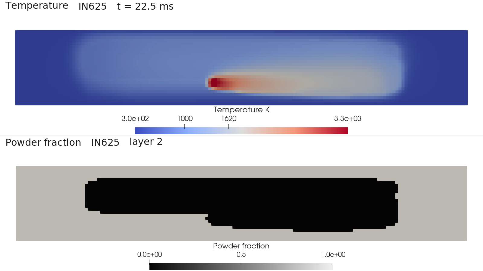
createScanPath writes rotated raster paths. runLayers cycles through those paths, creates layer0, layer1, and later directories, extrudes the mesh, maps the previous result, marks the new powder region, shifts the scan start time, decomposes, and runs each layer.

runLayers deletes and recreates existing layerN directories. Preserve results before rerunning.

Outputs

Open the reconstructed layer directories in ParaView to visualize the temperature, solid fraction, powder fraction, and heat-source fields across the deposited layers.

Top-surface temperature and powder fraction during the second layer at 22.5 ms. Powder fraction varies from black at 0 to light gray at 1; the black track identifies material consolidated by the moving heat source.

Plot solidification data

Set enabled true for solidificationData in system/controlDict before running the case. Each layer then writes its solidification events, and reconstructSolidificationData combines the processor files within the corresponding layer directory. From the base case, plot both layers on one CET diagram:

plotCET layer0 layer1

This creates CET_curve.png in the base case directory. Each plotted point gives the thermal-gradient magnitude and isotherm velocity for a recorded solidification event.

Run an ExaCA microstructure simulation

Set enabled true for the ExaCA Function Object in system/controlDict before running the case. Each layer then writes temperature events, and reconstructExaCAData creates these files:

layer0/ExaCA/time-temperature.csv
layer1/ExaCA/time-temperature.csv

The supplied ExaCA/input.json lists both files in TemperatureData.TemperatureFiles with paths relative to the base case. Launch ExaCA from that directory so the layer paths and output path resolve correctly:

mpirun -np <nProcs> /path/to/ExaCA ExaCA/input.json

ExaCA reads the layerwise temperature histories and writes the explicit microstructure result under ExaCA/. Runtime mesh redistribution must remain disabled while the ExaCA Function Object is active.

To write melt-pool dimensions for this case, enable meltPoolDimensions before running the layers and then use plotDimensions layer0 layer1. The complete Function Object configuration and plotting workflow are given in Write and plot melt-pool dimensions.