Heat-source Calibration

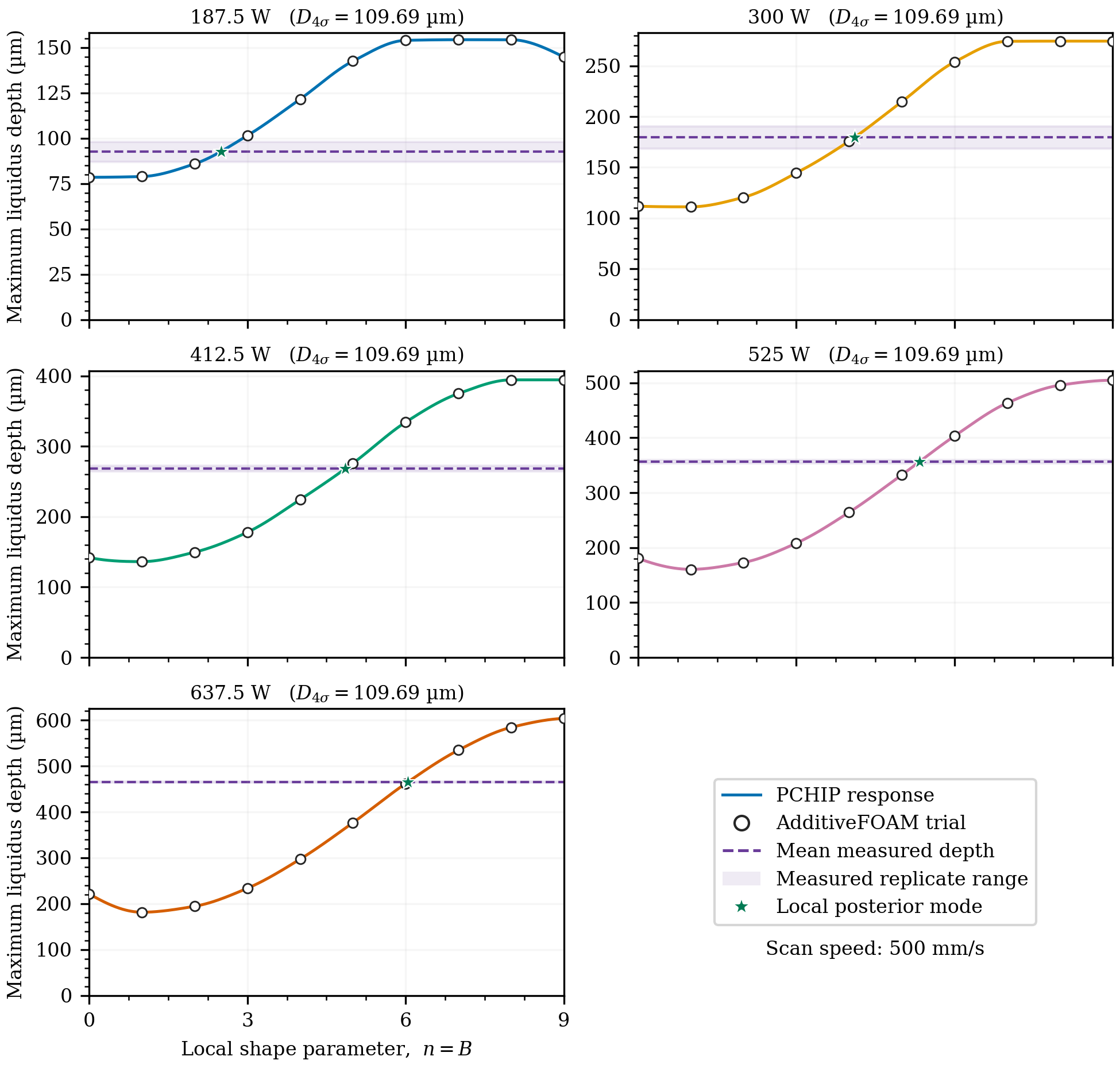
The calibration uses measured melt-pool depths from five SS316L single tracks on a bare plate. AdditiveFOAM response trials infer one local axial-shape value per power before fitting the nSlope–nIntercept relation.

Local AdditiveFOAM response curves. Each condition compares trial simulations with its two measured liquidus depths and identifies the local posterior mode.

Physical setup

• SS316L properties from $ADDITIVEFOAM_ETC/materials/SS316L.cfg.
• Five 2 mm single tracks on a bare plate at 500 mm/s.
• Incident powers from 187.5 W through 637.5 W.
• A 67-by-67 tabulated circular-Gaussian profile with 2.5 µm spacing.
• Profile D4Sigma of 109.69 µm.
• A projected heat source with a tabulated profile, exponential projection, configured depth 20 µm, and a liquidus reference depth.
• Kelly cylinder absorption with eta0 0.27, etaMin 0.27, and aspectRatioSwitch 0.
• Thermal-only trial cases with nOuterCorrectors 0.
• Eight MPI ranks per AdditiveFOAM simulation.

The experimental data in experiments.yml are:

Power (W)	Speed (mm/s)	Measured liquidus depths (µm)
187.5	500	87.05, 98.10
300.0	500	168.57, 190.67
412.5	500	272.19, 264.07
525.0	500	359.24, 353.71
637.5	500	464.25, 467.01

Run

Copy the tutorial to a writable run directory and launch the campaign:

cp -r "$ADDITIVEFOAM_TUTORIALS/heatSourceCalibration" \
  "$FOAM_RUN/heatSourceCalibration"
cd "$FOAM_RUN/heatSourceCalibration"
calibrateHeatSource --config config.yml

The campaign writes cases and results beneath its run directory, so use the writable copy shown above. If eight MPI ranks are unavailable, change template/system/decomposeParDict before starting.

The campaign evaluates nIntercept = 0,1,...,9 for all five experiments, for a total of 50 AdditiveFOAM simulations. Saved trial results allow the command to resume an interrupted campaign.

Important inputs

File	Purpose
config.yml	Paths, profile registration, trial design, deterministic posterior integration, global fit, and report settings
experiments.yml	Power, speed, profile name, and repeated measured depths
template/	AdditiveFOAM case rendered for each condition and trial
template/constant/beam_profile.txt	Normalized tabulated circular-Gaussian planar profile
template/constant/heatSourceDict	Kelly absorption and projected-source configuration
template/system/decomposeParDict	Eight-rank domain decomposition

Projected source template

The template contains:

sources
{
    beam
    {
        path            scanPath;
        widthReference  D4Sigma;
        D4Sigma         <<D4Sigma>>;
        depthReference  isotherm;
        isotherm        <<isotherm>>;

        absorption
        {
            model               Kelly;
            eta0                0.27;
            etaMin              0.27;
            aspectRatioSwitch   0.0;
            geometry            cylinder;
        }

        heatSource
        {
            model       projected;
            depth       20.0e-6;
            nPoints     (10 10 10);

            profile
            {
                model   tabulated;
                file    "beam_profile.txt";
            }

            projection
            {
                model       exponential;
                nSlope      0.0;
                nIntercept  <<nIntercept>>;
            }
        }
    }
}

For each trial, nSlope remains zero and <<nIntercept>> is the calibrated parameter. The other placeholders select the profile diameter and SS316L liquidus. The configured 20 µm depth is the minimum applied source depth.

Workflow

For each power condition, the command:

1. Copies template/ to campaign/cases/<condition>/nIntercept<trial>/.
2. Copies the named profile and renders the experimental parameters.
3. Runs the ten trial cases with ./Allrun on eight MPI ranks.
4. Extracts the maximum liquidus melt-pool depth from each trial.
5. Builds the response curve and local posterior.

The five local posterior modes are fitted to the global nSlope–nIntercept relation with uncertainty weighting and a soft_l1 loss. One thousand bootstrap refits propagate the local uncertainty to the response band.

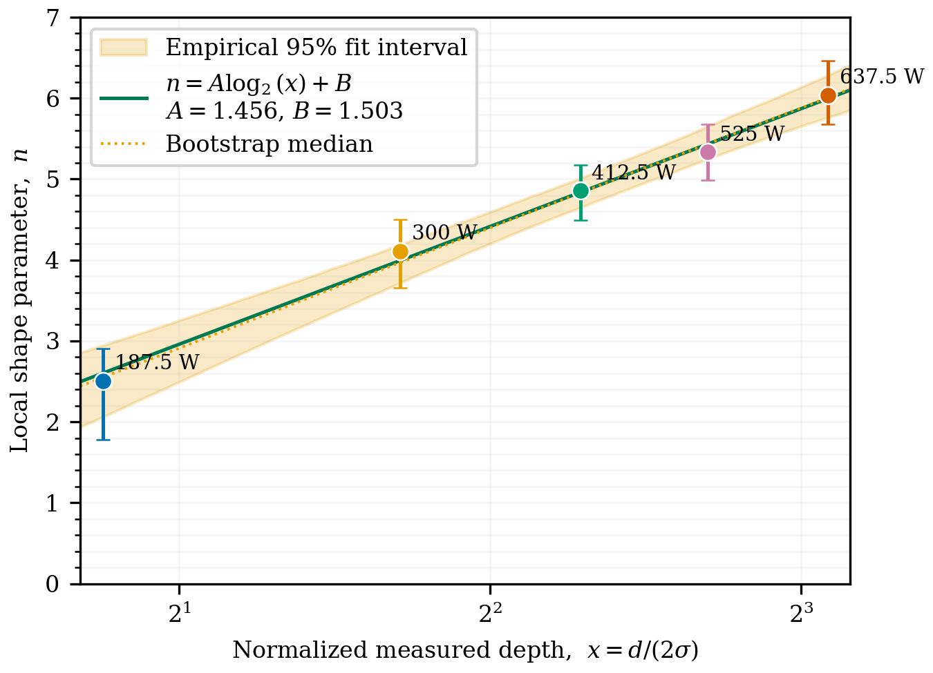
The global fit maps 2*Depth / selected diameter to the projected-source shape value using the area-equivalent D4Sigma = 109.69 µm.

Outputs

campaign/
├── cases/
│   └── P187p5_V500_measured_beam/
│       ├── nIntercept0/
│       ├── nIntercept1/
│       └── ...
├── simulations.yml
├── calibration_state.yml
├── calibration_fit.yml
└── reports/
    ├── calibration_report.pdf
    └── calibration_summary.csv

Successful trial directories retain their rendered inputs, solver log, post-processing output, and metrics.yml. With keep_successful: false, processor and numeric time directories are removed after the depth is recorded.

Apply the fit

Read nSlope and nIntercept from campaign/calibration_fit.yml and insert them into the projected source:

projection
{
    model       exponential;
    nSlope     <fitted-nSlope>;
    nIntercept <fitted-nIntercept>;
}

See Projected Heat-source Calibration for the equations and configuration reference.