AMB2018-02-B Single Track

This is the recommended baseline and quick-start case. It represents the NIST AM-Bench 2018 IN625 single-track experiment with calibrated absorption and source dimensions.

IN625 top-surface temperature as the heat source traverses the AMB2018-02-B track. The black and white contours denote the 1410 K solidus and 1620 K liquidus, respectively.

Physical setup

• IN625 properties from $ADDITIVEFOAM_ETC/materials/IN625.cfg.
• One superGaussian source with k 2, dimensions (85 85 30) µm, absorptivity 0.33, and nPoints (10 10 10).
• A 195 W, 0.8 m/s scan path.
• Optional refinement configuration, disabled by default.
• Fluid flow disabled by nOuterCorrectors 0 in the supplied case.

The calibration is described by Knapp et al., “Calibrating uncertain parameters in melt pool simulations of additive manufacturing”.

Run

cp -r "$ADDITIVEFOAM_TUTORIALS/AMB2018-02-B" "$FOAM_RUN/AMB2018-02-B"
cd "$FOAM_RUN/AMB2018-02-B"
./Allrun

The solver log should report approximately 33% of the active incident power as absorbed when the constant model is used and the source is fully contained by the domain.

Important inputs

File	Purpose
constant/heatSourceDict	Absorption, source distribution, sampling, and optional AMR
constant/scanPath	Beam position, power, and speed
constant/dynamicMeshDict	OpenFOAM topology changer
system/blockMeshDict	Base mesh
system/fvSchemes	Defaults to Euler
system/fvSolution	Defaults to the explicit temperature path

Workflow

Allrun generates the mesh, decomposes the case, runs additiveFoam in parallel, reconstructs the OpenFOAM fields, and invokes the ExaCA and solidification-data reconstruction utilities. The latter utilities produce output only when their corresponding Function Objects are enabled in system/controlDict.

Outputs

Open the reconstructed case in ParaView to visualize temperature, phase fraction, velocity, pressure, and heat-source fields. The following workflows produce quantitative outputs from the same case.

Plot absorbed power

additiveFoam writes the volume-integrated absorbed power to log.additiveFoam at every time step. From the case directory, plot that history with:

plotPower

The utility reads the time and absorbed power entries from the solver log and creates power.png. For the constant absorption model used by this case, the plotted value is approximately 0.33 multiplied by the active 195 W incident power while the heat source is fully contained within the domain.

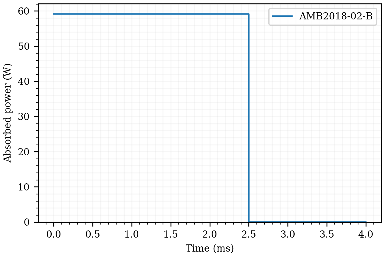
Output from plotPower. The constant-absorption model deposits approximately 59.1 W while the 195 W source is active and fully contained by the domain.

Write and plot melt-pool dimensions

Use this workflow to obtain melt-pool length, width, and depth as functions of time. Before running a fresh case copy, open system/controlDict and enable meltPoolDimensions:

meltPoolDimensions
{
    libs ("libadditiveFoamFunctionObjects.so");
    type          meltPoolDimensions;
    enabled       true;
    scanPathAngle 0;
}

With no isoValues entry, the Function Object writes both the IN625 solidus and liquidus isosurfaces from thermoPath. Run the case:

./Allrun

The CSV time histories are written under postProcessing/meltPoolDimensions/. Create the dimension plot from the case directory:

plotDimensions

The resulting melt_pool_dimensions.png contains length, width, and depth for each recorded isovalue.

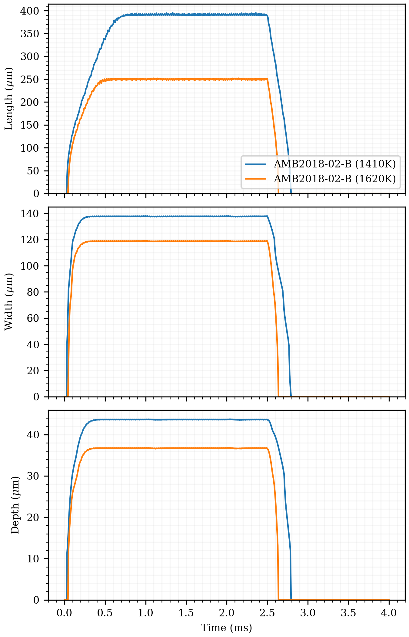
Output from plotDimensions. Blue denotes the 1410 K solidus isotherm and orange denotes the 1620 K liquidus isotherm.

Write solidification data and plot CET curves

Use this workflow to record cooling rate, thermal gradient, and isotherm velocity when material cools through the liquidus. In a fresh case copy, enable solidificationData in system/controlDict and set box to the physical region in which events should be collected:

solidificationData
{
    libs ("libadditiveFoamFunctionObjects.so");
    type      solidificationData;
    enabled   true;
    box       (-1 -1 -1) (1 1 1);
    isoValue  1620;
}

Run the case with ./Allrun. Each MPI process writes its events separately, and the final reconstructSolidificationData call in Allrun combines them into:

solidificationData/solidification-data.csv

Plot thermal-gradient magnitude against isotherm velocity from the case directory:

plotCET

This creates CET_curve.png. The plotted coordinates are the quantities commonly used to evaluate columnar-to-equiaxed transition criteria.

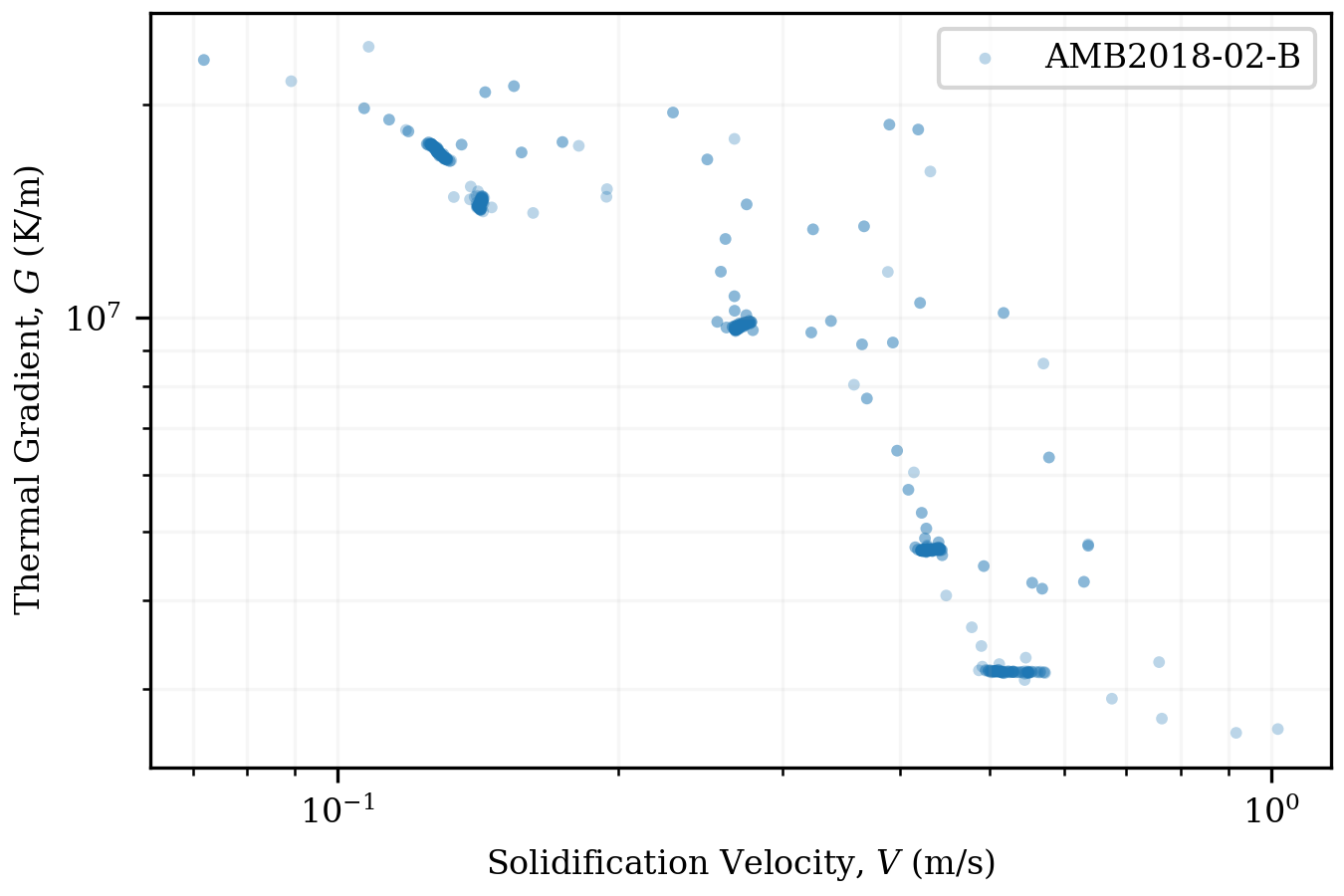
Output from plotCET. Each point is a liquidus-crossing event written by the solidificationData Function Object.

Create ExaCA temperature histories

Use this workflow to generate explicit temperature histories for an ExaCA microstructure simulation. In a fresh case copy, enable ExaCA in system/controlDict:

ExaCA
{
    libs ("libadditiveFoamFunctionObjects.so");
    type      ExaCA;
    enabled   true;
    box       (-5e-5 -0.00025 -0.0002) (0.0025 0.00025 0);
    dx        2.5e-6;
    isoValue  1620;
}

box defines the microstructure-sampling region, dx is the Cartesian sampling spacing, and isoValue is the temperature used to identify melting and solidification. Run ./Allrun; its reconstructExaCAData step creates:

ExaCA/time-temperature.csv

The supplied ExaCA/input.json already reads that file through TemperatureData.TemperatureFiles. From the AdditiveFOAM case directory, launch an installed ExaCA executable with the desired MPI process count:

mpirun -np <nProcs> /path/to/ExaCA ExaCA/input.json

ExaCA reads the reconstructed melt and solidification events and writes the explicit microstructure result under ExaCA/. Runtime mesh redistribution must remain disabled while the ExaCA Function Object is active.